The following methodology applies to this publication – Student loans forecasts for England, financial year 2025-26 only. Methodologies relating to previous publications can be found at this link Archive Timeline - UK Government Web Archive (opens in new tab).
Income Contingent Repayment (ICR) student loans are provided by Government to higher education students and some further education students to cover course fees and living costs while they are studying. They were first introduced in the UK for new undergraduate students in 1998, at the same time as tuition fees. Prior to 1998, university students were provided funding by Government through a mixture of grants and, from 1990, mortgage-style loans that were available to help with living costs. Mortgage-style loans are not covered in this publication.
Each of the four constituent countries of the UK now have their own student loan policies, but only students who are eligible through Student Finance England (SFE) are considered in this publication. These are loans issued to English-domiciled students at UK providers and a small number of students of other residencies that attend learning providers in England. A summary timeline of income-contingent repayment loans is available in Table 1.1 below.
Table 1.1: Income Contingent Repayment loan timeline: England
1998
Plan 1 loans introduced for new UK domiciled undergraduate students, to cover living costs.
Annual tuition fee of up to £1,000 also introduced in 1998 Teaching and Higher Education Act.
2006
Maximum annual tuition fee limit increased to £3,000 for new full-time undergraduate entrants.
Tuition fee loans introduced to meet the costs of tuition for new full-time undergraduates.
Maintenance grants introduced for new full-time undergraduate entrants on lower incomes.
EU domiciled students became eligible to take out tuition fee loans.
Repayment term changed to 25 years for new entrants, rather than ending at age 65.
2012
Plan 2 loans introduced for new entrants.
Maximum annual tuition fee limit increased to £9,000 for new full-time undergraduate entrants.
New eligible part-time undergraduates subject to maximum tuition fee limit of £6,750 and entitled to fee loans for the first time to meet the full costs of their tuition.
2013
Advanced Learner Loans introduced for students aged 24+ on designated Level 3-4 further education courses in England, on the Plan 2 system. Advanced Learner Loans Bursary Fund introduced.
2016
Plan 3 loans introduced for new students taking postgraduate Master’s courses, who could borrow up to £10,000 over the length of their course.
Maintenance grants replaced by additional loans for living costs for new full-time undergraduate entrants on lower incomes.
Advanced Learner Loans and Bursary Fund extended to students aged 19-23 and to Level 5-6 designated courses.
2017
Nursing, midwifery and most allied health students become eligible for student loans, in place of receiving NHS bursaries.
Maximum annual tuition fee limits increased for new entrants and continuing students who started their courses on or after 1 September 2012 (£9,250 for a full-time course, £6,935 for a part-time course).
2018
Plan 2 repayment threshold increased from £21,000 to £25,000. It had previously been announced that it would remain at £21,000 until April 2021.
Doctoral degree loans of up to £25,000 across the length of a borrower’s course introduced for new starters, on the Plan 3 system.
Loans for living costs introduced for new part-time undergraduates attending degree-level courses and level 5 pre-registration healthcare courses only.
2019
Plan 2 repayment threshold increased to £25,725 for tax year 2019-20, and was thereafter increased annually in-line with average earnings growth figures published by the Office for National Statistics (ONS) until subsequent freezes were announced.
2020
Plan 3 repayment threshold remains at £21,000 until April 2022.
2021
Student Finance support for EU Domiciles withdrawn.
2022
Plan 3 repayment threshold remains at £21,000 until April 2023
Plan 2 repayment threshold remains at the financial year 2021-22 level of £27,295 until April 2025 increasing annually with RPI (Retail Price Index) rather than earnings thereafter
Interest rate for plans 2 and 3 capped at 7.3% for academic year 2022/23 in line with forecast prevailing market rate
2023
Plan 3 repayment threshold remains at £21,000 until April 2024
Plan 5 loans introduced for new entrants starting from 1st August 2023, with repayment threshold at £25,000 until April 2027 (increasing annually with RPI thereafter), a repayment term of 40 years and a rate of interest in and after study of RPI+0%
Maximum annual tuition fee limits frozen at 2022/23 levels for the 2023/24 and 2024/25 academic years for new and continuing undergraduate students (£9,250 for full-time courses, £6,935 for part-time courses)
2025
Plan 3 repayment threshold remains at £21,000 until April 2026
Plan 2 repayment threshold freeze ended in April 2025. Threshold increased to £28,470 reflecting RPI outturns.
Maximum annual tuition fee limits increased for new and continuing undergraduate borrowers in the 2025/26 academic year to £9,535 for full-time courses and £7,145 for part-time courses at providers with a TEF award.
2026
Plan 2 repayment threshold to be frozen at 2026-27 levels until April 2030, when it will return to increasing with RPI, as announced at the 2025 Autumn Budget.
Plan 3 repayment threshold remains at £21,000 until April 2027.
Plan 2 and Plan 3 interest rates capped at 6% for the 2026/27 academic year.
Student loans are issued and administered by the Student Loans Company (SLC) on behalf of the Government and the devolved administrations in the UK. The Department for Education produces forecasts for its outlay on, and the repayments it expects to receive from, the English student loans that it is responsible for. These forecasts are audited by the National Audit Office (NAO) annually and are subject to the Department for Education’s quality assurance framework for business-critical models. The forecasts are scrutinised and cleared by quarterly internal Models and Funding Boards before they are used in financial planning, policy development and to value the loans that have been issued in its annual accounts. The forecasts presented in this publication are produced across multiple models, as follows:
Entrant borrowers model – this model forecasts the annual growth in the number of full-time undergraduate loan borrowers in year one of their course, studying at providers eligible to charge for the maximum annual tuition fee loan amount. This makes up the majority of the full-time undergraduate loan borrowing population. The growth rates from this forecast are applied to the latest year of outturn SLC data (academic year 2024/25) in the student loan outlay model.
Student loan outlay model – this model produces forecasts of loan outlay on higher education ICR loans issued to undergraduate and postgraduate students.
Student loan earnings model – this model produces forecasts for the future earnings of higher education ICR loan borrowers.
Student loan repayments models – separate undergraduate and postgraduate models produce forecasts for the future repayments that will be made by higher education ICR loan borrowers.
Advanced Learner Loans model – this model produces forecasts for loan outlay and repayments that will be made on Advanced Learner Loans, which are available for some further education courses.
This document provides information on these models, including the methodology, data sources and assumptions used in producing the forecasts.
With the exception of the Lifelong Learning Entitlement (LLE) (opens in new tab), these forecasts incorporate existing government policy announced by April 2026, which is when this forecast was approved by DfE. From September 2026, learners will be able to apply for LLE funding for courses and modules commencing from January 2027 onwards. The introduction of the LLE, and any other changes to student loan eligibility, loan amounts, or terms and conditions, if implemented by Government after 27 April 2026, are not accounted for in the forecasts in this publication. The policy to cap interest rates at 6% in academic year 2026/27 for Plan 2 and Plan 3 loans is included in these forecasts.
DfE’s higher education (HE) undergraduate (UG) entrant borrower model forecasts the annual growth in full-time undergraduate Student Finance England loan borrowers commencing a new course. The growth rates from this forecast are applied to the latest year of outturn SLC data (academic year 2024/25) in the student loan outlay model, which informs the department’s financial accounts of Student Finance England student loan outlay.
Courses eligible for public funding via student loans may be delivered by a lead provider or by a partner institution (franchised provider) on behalf of the lead provider. Lead providers are the higher education institutions students register with; they retain overall responsibility for a course delivered, including responsibility for its quality, standards, and oversight, even when that course is delivered under a subcontractual (franchised) arrangement. Franchised providers are the partner organisations that run courses on behalf of lead providers under subcontractual arrangements. At present, lead providers must register with the Office for Students so that their students can access student loans, but franchised providers need not.
Growth in franchised provision has accelerated in recent years. In response, the Department launched a sector-wide engagement programme in 2025 to address concerns of fraud, abuse of public money and poor value for students. To capture this growth accurately and estimate how the Department’s engagement will affect it, the entrant borrower model forecasts the growth in franchised and direct provision separately.
Scope
The UG entrant borrowers forecast covers student entrants who are entitled to both tuition fee and maintenance loans, have taken out a SFE student loan and are studying a level 4, 5 or 6 course. These students are registered with an Approved (fee cap) (opens in new tab)providers in England or a Higher Education provider in Scotland, Wales and Northern Ireland; Approved (fee cap) providers are eligible to charge the maximum annual tuition fee loan amount (£9,790 in academic year 2026/27).
The following borrowers are excluded from the entrant borrowers forecast:
Borrowers whose loans are administered by the Devolved Administrations.
Borrowers who are not eligible to take out a maintenance loan according to the regulations (referred to as partial support).
Borrowers studying at Approved providers in England (or being charged the Approved fee amount).
Borrowers who are not in the first year of their course (referred to as returning students).
Undergraduate SFE loan borrowers that fall in group 3-5 are captured separately within DfE’s higher education student loans outlay model.
The UG entrant borrower model does not cover any entrants that have not taken out a Student Finance England student loan. The population in scope includes a small number of EU nationals with pre-settled residency status who are entitled to Student Finance England loans as a result of the UK–EU Withdrawal Agreement. This small group of entrant borrowers are forecast separately from the rest of the undergraduate borrower population because their numbers will decrease substantially in 2026, once the EU pre-settled status ceases to exist.
SLC administrative data inclusive 2024/25, as of 31 August 2025.
Entrant borrowers
The historical number of entrant borrowers in each academic year is derived from administrative data obtained from the Student Loans Company. A borrower is counted if they are on the first year of a new course, has taken out a loan from SFE (fee and/or maintenance) and fits the scope of the target population (see “Scope” section above). Borrowers are aggregated by academic year (2013/14-2024/25), sex (male, female), age group (18 and under, 19, 20, 21-24, 25-34 and 35 and over), and provision type (direct provision or franchised provision). Direct provision entrants are entrants whose course is run by the lead provider, while franchised provision entrants are entrants whose course is run by a subcontracted provider that delivers the course on the lead provider’s behalf (see Franchising adjustment forecast, below for more detail).
Direct provision borrower counts are divided by the number of people in the general population to obtain the proportion of the population that has taken out a loan in each age-sex subgroup - we refer to this proportion as the borrower rate. Franchised provision counts are modelled without conversion into borrower rates to reduce volatility in the fitted timeseries. The latest data from the Student Loans Company has an effective date of 31 August 2025 and contains borrowers for academic years up to and including 2024/25.
Population
It is assumed that ONS population data for England are a suitable proxy for the underlying population of the Student Finance England borrower population. ONS population estimates and projections are aggregated by sex (male, female) and age group (18, 19, 20, 21-24, 25-34 and 35-60). These estimates and projections are used as the denominator population count for each age-sex group of borrowers to obtain the borrower rate. Population counts for 18-year-olds are used as the denominator for borrowers aged 18 and under, and population counts for people aged 35-60 are used for borrowers aged 35 and over, as borrower numbers for people aged under 18 and over 60 are very small.
Main scheme applicants
Main scheme applicants refer to applicants who apply through the UCAS application system by the end of June (exact date varies from year to year). January deadline applicants are a subgroup of main scheme applicants who apply by the interim deadline, in January (date also varies annually). January deadline applicants make up the majority of main scheme applicants, but not all of them. The entrant borrowers model uses the January deadline figures to predict the number of borrowers in the second forecast year (2026/27), because at the time of the model update included in this publication, only the January deadline data had been published. These numbers do not include applicants who applied for the first time through UCAS clearing or applicants who made applications directly to providers.
The entrant borrower model uses these lead indicator applicant figures to predict the number of direct provision borrowers expected in the second forecast year, using the historical trend in the annual ratio between applicants and borrowers. In the current version of the forecast, this data was used for estimating the borrower numbers of entrants aged 20 or under in the second year of the forecast.
Main scheme accepted applicants
The entrants model uses UCAS end of cycle acceptances data that cover the number of applicants that were accepted through UCAS main scheme or UCAS clearing application systems. It uses these lead indicator figures to predict the number of borrowers in the first year of the forecast in direct provision groups.
Sex and gender classifications
The Student Loans Company records borrower’s sex and provides two options (male and female). UCAS data reports applicant’s gender and provides several options. While these two classifications do not completely align, using gender from the applicant and accepted applicant data as a proxy for sex in the borrower data will have minimal impact on the overall accuracy of the forecast and is deemed valid for the current purpose. Instances where the gender is not ‘woman’ or ‘man’ in UCAS data are combined with female applicants or accepted applicants because females account for the largest number of entrants. This assumption has made minimal impact to the forecast historically and is continually being reviewed.
Methodology
The entrant borrowers model forecasts annual growth in entrant borrowers over a six-year period. Forecasts are run separately for each age group, sex and provision type group, or stratum. Before they are modelled, direct provision figures are converted to borrower rates. Franchised provision counts are modelled without conversion.
Model structures
Each direct provision stratum is forecast using either a one-stage or a two-stage model structure. A one-stage structure projects the historical trend in borrower rates or borrower counts from SLC data forward in time to the end of the forecast period. A two-stage structure first predicts the number of borrowers in the first 1 to 2 years of the forecast using the historical trend in the ratio between borrower numbers and UCAS lead indicator figures. These predictions are appended to the historical timeseries of borrower data, and the combined trend is fitted and projected forwards over the remaining 4-5 years of the forecast in stage two, depending on whether one or both of the lead indicator data sources were used.. These lead-indicator models capture the predictive power of the UCAS data, including the uncertainty in how UCAS figures have historically translated entrant borrower numbers in SLC data. The model does not assume that a single model structure will perform well across all age/sex/provision-type strata, so initially all strata are fitted with both structures.
Franchised provision strata are forecast using only a one-stage model to obtain a forecast that reflects the potential growth that would have occurred had the Department not taken engagement action in 2025. The impacts of the enforcement action on future entrant numbers are modelled separately and the reduction of entrants expected is applied in the outlay model.
Forecasting approaches
The model also does not assume that a single fitting approach will perform well across all strata either, so each structure (in all strata) is also fitted with a range of fitting approaches. Both the two-stage and trend-only forecasts are run using exponential smoothing (ETS) models and random walk models, with and without a drift term.
The lead indicator models, run in the first stage of the two-stage model, are fitted with an ETS model and a random walk model without drift. The latter is used when there is a high level of uncertainty regarding the direction of the trend, or the back series is noisy.
Exponential smoothing (ETS) models
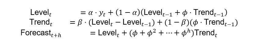
ETS models forecast future borrower rates or counts by applying weighted averages to past observations, giving greater emphasis to recent data so that new data influences the forecast more strongly than older ones. This approach allows the model to adapt quickly to changes while still considering historical patterns. ETS models can dampen trends, meaning they gradually flatten the slope of the forecast over time to avoid unrealistic long-term growth or decline. They can also control how responsive the forecast is to new data when setting the trend component, and how quickly the forecast updates its estimate of the current level based on new observations. These are varied using Phi (φ), beta (β) and alpha (α) parameters, respectively. A model with low values of α and β reacts slowly, favouring stability, whereas high values favour reactivity. Lower values of φ produce stronger damping, whereas higher values allow the trend to persist for longer.
For an ETS model with additive trend and dampening:
Data is fitted with ETS variants, with different β (beta) values, designed to vary how quickly the trend responds to new data:
Short-term (β = 0.7) highly responsive
Medium-term (β = 0.4): moderately responsive
Long-term (β = 0.1): less responsive
In all three ETS variants, alpha (α) is fixed at 0.7, ensuring that the level component remains stable and avoids introducing artificial growth or decline in the first year that is forecast. This choice reflects the aim for a smooth, realistic transition from historical data or lead indicator prediction to forecast. Phi (φ) is fixed at 0.9, which represents a modest amount of dampening. Together, these settings allow us to balance responsiveness and stability across different forecasting horizons and preserve the ability to explain the drivers of the forecasts.
The lead indicator models used to predict borrower numbers from UCAS figures in the first one to two years of the forecast are fit with an ETS model that responds quicky to new data when setting the level (alpha 0.7), reacts moderately when setting the trend (beta 0.5) and applies minimal dampening (phi 0.95).
Model selection
The best forecast for each stratum is chosen based on its performance in back testing relative to the other candidate models, analytical judgement and policy intelligence. Thus, the forecasts of some strata may be informed by UCAS lead indicator data because that data has predictive power - while others may be driven only by historical trends in borrower rates, because the lead indicator data performs worse or more noisily than the historical trend alone and risks producing a less accurate forecast. Likewise, some forecasts may have been produced with a long-term ETS model because it is assumed that recent growth is equally informative of the future as growth observed in earlier years, while others may be fitted with a medium-term ETS model - which puts less weight on the earliest years than the long-term model - because those earlier years are deemed to be less representative of future growth, for example due the trend changing. A random walk model is chosen when there is no obvious trend in the historical data or a high level of uncertainty regarding direction of growth.
The models chosen for the direct provision section of the forecast in this publication are shown in Table 2.1. All franchise provision strata are fitted with a medium term ETS, one-stage model.
Table 2.1: Models chosen for the direct provision section of the forecast
Stratum
Forecast Year 1
Stratum
Forecast year 2
Stratum
Approach taken to fit
Age 18 and under, Females
Predicts borrowers using the historical ratio between borrowers and total accepted applicants
Age 18 and under, Females
Predicts borrowers using the historical ratio between borrowers and main scheme applicants who applied by the January deadline.
Age 18 and under, Females
ETS long term
Age 18 and under, Male
Age 18 and under, Male
Age 18 and under, Male
Age 19, Females
Age 19, Females
Age 19, Females
Age 19, Males
Age 19, Males
Age 19, Males
Age 20, Females
Predicts borrowers based on the projected ratio between borrowers and accepted applicants (main scheme and direct-to-clearing routes only) using ETS lead indicator model.
Age 20, Females
Age 20, Females
Age 20, Male
Age 20, Male
Age 20, Male
ETS medium term
Age 21-24, Female
Age 21-24, Female
No lead indicator, as UCAS main scheme applicant data is not predictive of borrower numbers in these strata.
Age 21-24, Female
ETS long term
Age 21-24, Male
Age 21-24, Male
Age 21-24, Male
Age 25-34-Female
Age 25-34-Female
Age 25-34-Female
ETS medium term
Age 25-34-Male
Predicts borrowers using the historical ratio between borrowers and accepted applicants (main scheme and direct-to-clearing routes only) using random walk lead-indicator model.
Age 25-34-Male
Age 25-34-Male
Age 35 and over, Females
Predicts borrowers using the historical ratio between borrowers and accepted applicants (main scheme and direct-to-clearing routes only), projected with an ETS lead indicator model.
Age 35 and over, Females
Age 35 and over, Females
Random walk
Office for Students (OfS) registration
Since academic year 2019/20, providers in England (offering higher education courses) that wish to charge the maximum tuition fee amount are required to register with the OfS under the Approved (fee cap) (opens in new tab) category (opens in new tab). The entrant borrowers forecast captures the growth in entrants at lead providers that registered as Approved (fee cap) by 31st August 2025. The forecast does not include entrants at providers that are yet to register as Approved (fee cap). The entrant borrowers model does not include the students at Approved providers; these loan borrowers are captured within DfE’s higher education student loans outlay model.
NHS Long-term Workforce Plan
The NHS Long-term Workforce plan (opens in new tab) aims to significantly expand the number of training places for healthcare courses over the next decade, including medicine and dentistry, nursing, midwifery and subjects allied to medicine, with a particular focus on areas facing staff shortages. The impact of these additional training places on the number of borrowers expected over the forecast period was estimated together with the Department of Health and Social Care (DHSC) and is included in this forecast.
Franchising adjustment forecast
The Department has undertaken a programme of sectoral engagement to address the risk about fraud, abuse of public money and poor value for students caused by the rapid growth of franchised provision where this is not supported by sufficiently robust oversight and controls.
The behavioural response impact of this engagement action on future entrant numbers was estimated using a two-part microsimulation model. In the first stage of the model, franchise arrangements are allocated to one of four strategies (continued growth, maintaining their current cohort size, shrinking over time, or ceasing recruitment altogether). In the second stage of the model, the impacts of these strategy choices are then applied to future entrants, who may remain in franchised provision, be displaced into non-franchised HE provision or may choose not to enter HE.
The number of students in each academic year estimated to no longer enter HE due to reduced capacity at franchised providers forms the ‘franchising adjustment’ forecast. This franchising adjustment forecast is used in the outlay model to adjust the future borrower population, removing the appropriate number of entrants from future franchised provision.
This forecast does not yet include impacts of the Department’s requirement for most franchised providers with more than 300 students to register with the Office for Students.
Forecast
Table 2.2 shows the forecast for full-time undergraduate entrant loan borrowers at Approved (fee cap) providers in England and providers in the Devolved Administrations eligible to charge the maximum loan amount, before and after policy amendments are applied.
Table 2.2: Forecast for full-time undergraduate entrant loan borrowers at Approved (fee cap) providers in England and Higher Education providers in the Devolved Administrations
Academic Year
Direct provision (before additions)
Franchised provision (before removals)
Total forecast before policy additions and removals
Total forecast incl. additions and removals
Annual growth rate, total forecast incl. additions and removals
2025/26
364,800
70,000
434,800
429,900
1.9%
2026/27
372,700
75,400
448,100
441,700
2.7%
2027/28
373,200
80,700
453,900
445,800
0.9%
2028/29
374,000
85,800
459,800
451,900
1.4%
2029/30
376,900
90,900
467,800
459,800
1.7%
2030/31
378,400
95,900
474,300
465,500
1.2%
Long-term forecasts
Beyond the six-year forecasting period, growth in loan-eligible entrants is forecast using ONS population projections, weighted according to the age make-up of the borrower population. This forecast is used in the student loans outlay and the student loans repayment models. Separate projections are produced for full-time and part-time undergraduate entrants, and for Master’s and Doctoral entrants. To obtain these growth rates, ONS principal population projections for each age are first converted into cumulative growth rates, with the final year of the short-term forecast as the baseline (i.e. academic year 2030/31). For undergraduates, these are then weighted according to the distribution of age observed in the last forecast-year of the Student Loans Outlay Model with the effective date of November 2024. Student Loans Outlay Model sampling (which the forecast is dependent on) identifies age at course start date of the loan-borrowing entrant from the difference in years between the date of birth and the course start date. For Master’s and Doctoral entrants, the growth rates are weighted by the age distribution of borrowers in SLC data for academic year 2019-2021. At the time of this analysis, the effective date of the SLC data was April 2023. For each study level, weighted growth rates are then summed across age to obtain total cumulative growth (i.e. for each of the student population), from which the year-on-year growth is then calculated.
Data quality
The nature of any forecast is inherently uncertain and dependent on the quality of the source data, modelling methodology and model assumptions. The entrant borrowers model uses published data from ONS and UCAS as well as administrative data from the Student Loans Company to forecast full-time undergraduate entrants.
ONS Population Estimates and Projections
ONS population estimates and projections used in the short‑term and long‑term entrant borrower models are fully accredited official statistics and the primary population statistics used across Government. ONS figures are produced as mid‑calendar‑year estimates, whereas entrant borrower forecasts are run on an academic‑year basis (generally September to August). While this misalignment may have a small impact on forecast accuracy, ONS population projections are considered sufficiently robust for modelling purposes, as most full‑time undergraduate entrants commence study in the first calendar year of the academic year, which broadly aligns with the population data.
Data quality guidance for population projections (opens in new tab) and estimates (opens in new tab) is published by ONS. Short-term principal projections are largely considered reliable; given that the entrant borrowers model only forecasts over a six-year period, this increases confidence in the base population which forecast entrant are modelled from. ONS do not make any predictions of future political or economic changes that could affect population numbers.
UCAS data
The model uses open access statistical reports published by UCAS on higher education applications and acceptances at various points in the cycle. UCAS voluntarily apply (opens in new tab) the Code of Practice for Statistics to their statistical releases and their releases are considered reliable.
Limited historical coverage following the £9,000 tuition fee reform
The entrant borrowers model relies on a relatively short and recent historical series, which increases forecast uncertainty and sensitivity to unusual movements in the data. This is because data prior to funding reforms in academic year 2012/13 are not representative of future borrower behaviour, given the substantial changes to tuition fee levels and student finance arrangements following the increase to £9,000 per year. The use of post‑reform data only improves relevance but reduces the number of usable observations, making the model more exposed to short‑term fluctuations, including those driven by policy changes and the Covid‑19 pandemic.
Impact of international students on the entrant loan borrowing population
No assumptions are explicitly made regarding the growth of international students and what impact it might have on the growth of the SFE loan-borrowing entrant population. Given the many factors that influence international applicant demand, there are limited sources of forecasts. However, we continue to monitor UCAS and HESA data. Recent policy changes mean future growth is uncertain; however, this is assumed to have little effect on the growth of domestic student entrants because international students account for a relatively small proportion of the full-time undergraduate student entrant population.
Entrant borrowers model uncertainties
There is uncertainty around provider capacity, including whether providers will be able to continue growing at the current rates and how long they will be able to continue growing for. Provider behaviour during the 2025/26 UCAS acceptance cycle suggests that at least some providers, such as those UCAS refers to as “high tariff” providers are trying to grow by making more acceptances than in previous years and accepting applicants earlier in the cycle than in previous years.
The postgraduate entrant borrowers model forecasts the number of postgraduate students expected to take out a Student Finance England postgraduate loan for a Master’s or Doctoral degree, over a six-year forecast period. The forecast borrower numbers are used in the Outlay model which informs the department’s financial accounts of Student Finance England student loan outlay.
Scope
The forecast covers entrant loan borrowers that have taken out a Student Finance England postgraduate loan and are registered at an HEI providers in England and the Devolved Administrations. These are students that are eligible for student loans because they have been ordinarily domiciled in England for at least 3 years before the start of their course. The population in scope includes a small number of EU nationals with pre-settled residency status who are entitled to Student Finance England loans as a result of the UK–EU Withdrawal Agreement. This small group of entrant borrowers are forecast separately from the rest of the postgraduate borrower population because their numbers will decrease substantially in 2026, once the EU pre-settled status ceases to exist.
Data
The data used for the forecast is provided by SLC throughout the year and contains aggregate numbers of postgraduate Student Finance England entrant borrowers taking out loans for Masters and Doctoral courses, for each academic year. The most recent data set has effective date of 31 January 2026 and includes academic years up to and including 2025/26. The SLC payment cycle can run for a year longer than the academic year does, as borrowers can apply up to 9 months after the day their course starts and courses can start at various points throughout the academic year. Because of this, academic years 2024/25 and 2025/26 figures are partial. Data for academic years up to and including 2023/24 are complete.
Methodology
The model first estimates the number of borrowers expected at the end of academic years whose payment cycles are not finalised. It calculates the growth between the end of January and the end of the payment cycle in the most recent academic year with complete data. The model then increases the borrower numbers in the incomplete academic years by that growth. These figures are then appended to the historical timeseries and modelled.
The Doctoral and Masters forecasts are constructed separately using an ETS model (for details see Exponential smoothing (ETS) models section), set to heavily weight recent data when setting the level and the trend of the forecast, and apply a small degree of trend dampening. The intent behind the model settings is to inform the forecast with the growth observed in the years following the Covid-19 pandemic, which saw unusually high level of growth across the HE sector. In both forecasts, alpha and beta are set to 0.9 and 0.7, respectively. Phi is set to 0.95 in the Master’s forecast and 0.9 in the Doctoral forecast. These parameter values are relatively high, meaning the model places strong emphasis on recent observations, ensuring forecasts are responsive to recent shifts. The forecast assumes that 73% of Master’s entrants will study on a full-time basis and 27% on a part-time, and that 62% of Doctoral students will study full-time and 37% part-time.
A small number of EU nationals with pre-settled status are added to these forecasts. These groups are expected to stay flat until 2026/27 based the growth observed in their numbers in the last 3 academic years. From 2026/27 the pre-settled status will no longer exist and therefore no new borrowers with pre-settled status will take out SFE loans. As a result, this group drops out the forecast.
Forecast
Table 3.1 Forecast for the post-graduate entrant loan borrowers at HE providers in England and the devolved administrations
Academic Year
Masters entrant borrower forecast
Annual growth
Doctoral entrant borrower forecast
Annual growth
2025/26
62,100
6.6%
2,700
9.6%
2026/27
65,100
4.8%
2,900
6.4%
2027/28
68,300
4.9%
3,100
6.1%
2028/29
71,300
4.4%
3,200
5.2%
2029/30
74,200
4.0%
3,400
4.4%
2030/31
76,900
3.7%
3,500
3.8%
Assumptions
The forecasts assume that no changes will be made to loan eligibility policies over the forecast period.
Payment cycles (and therefore borrower numbers) are deemed complete one year after the end of the academic year a borrower started their course on, based on the progression of borrower numbers in previous payment cycles.
The model assumes that growth across the most recent complete payment cycle is a good enough proxy for growth across payment cycles that are not yet complete.
The model assumes recent years (2023/24–2025/26 as of April 2026) are more representative of future demand than earlier years.
The model assumes no capacity constraints in postgraduate provision over the forecast period.
Uncertainties
The growth in the forecast is informed by a relatively small number of academic years, which makes the forecast inherently uncertain.
Masters and Doctoral loans are relatively new compared to undergraduate loans, having only been introduced in 2016/17 and 2018/19, respectively. There is uncertainty on whether borrower behaviour has yet stabilised.
Data quality
The model uses SLC administrative data to determine entrant borrower numbers. The DfE receives data reports on postgraduate loans from the Student Loans Company quarterly basis. SLC publishes a statement on its administrative sources (opens in new tab).
The student loan outlay model forecasts loan amounts that the Department for Education (DfE) expects to pay higher education students (and their providers) via the Student Loans Company (SLC).
A range of sub-models are used to capture the various loan types available to students. The loan products that outlay forecasts are produced for are:
Full-time undergraduate loans (Plan 2) – the loan system for students on full-time courses that started between September 2012 and 31st July 2023 and that are eligible for undergraduate student support funding, consisting of fee loans and maintenance loans.
Part-time undergraduate loans (Plan 2) – the loan system for students on part-time courses that are eligible for undergraduate student support funding. These first became available in September 2012, consisting of a tuition fee loan. From August 2018, maintenance loans were also available to some part-time students.
Full-time undergraduate loans (Plan 5) – the loan system for students on full-time courses that start on or after 1st August 2023 and are eligible for undergraduate student support funding, consisting of fee loans and maintenance loans.
Part-time undergraduate loans (Plan 5) – the loan system for students on part-time courses that start on or after 1st August 2023 and are eligible for undergraduate student support funding, consisting of fee loans and maintenance loans for some part-time students.
Postgraduate Master’s loans (Plan 3) – loans available to Master’s students to help cover fees and living costs. They were introduced in August 2016 and are on the Plan 3 repayment system.
Postgraduate Doctoral loans (Plan 3) – loans available to Doctoral students from August 2018 to help cover fees and living costs. They are on the Plan 3 repayment system.
Outlay forecasts for Plan 1 loans are no longer produced due to the negligible number of recipients expected in the academic year 2025/26, because most students who started a course before September 2012 have now completed those studies.
Eligible English-domiciled students are entitled to tuition fee and maintenance loans for courses that are eligible for undergraduate funding, and Master’s and Doctoral loans for courses that are eligible for postgraduate funding. Previous publications included a separate ‘EU borrower’ forecast, for EU domiciled students who were eligible to take out tuition fees loans only. In the 2021/22 academic year this student finance support was withdrawn following the UK’s exit from the EU and the residency status that defines this small group of borrowers with partial eligibility has changed. Partial eligibility covers those who do not have access to undergraduate maintenance funding but have access to postgraduate funding and undergraduate tuition fee-only funding. This group now comprises a mixture of:
EU nationals with pre-settled status,
EU, other EEA and Swiss nationals still eligible for tuition fee loans as a result of the Withdrawal Agreement, including Irish nationals who have not been domiciled in the UK for 3 years before starting studies,
Other residencies granted partial higher education support under the regulations.
This group is now labelled ‘Borrowers granted partial higher education support under the regulations’. Both this group and English domiciled students are entitled to the same amount for postgraduate loans, but the two groups are forecast separately to capture the difference in their expected growth. For further details on loans and eligibility, please see the Student Finance England practitioner website (opens in new tab).
whether they have a Teaching Excellence and Student Outcomes Framework (TEF) rating, and
whether they have an Access and Participation Plan (APP) approved by the OfS.
For the 2025/26 academic year, approved (fee cap) providers with an approved APP can charge higher fees for full-time students:
up to £9,535 with a TEF award, and
up to £9,275 without a TEF award.
If an Approved (fee cap) provider does not have an approved APP, they can only charge the basic fee amount:
up to £6,355 with a TEF award, and
up to £6,185 without a TEF award.
Providers registered in the Approved category are not subject to fee limits. However, students at these institutions are only eligible for student support up to the basic fee cap that applies to Approved (fee cap) providers.
Maintenance loans for eligible students depend on their location and household income (where a borrower applies for a means tested loan). The maximum maintenance loan for full-time Plan 5 borrowers living away from home and studying outside of London, in academic year 2025/26 is £10,544, as outlined in the financial memorandum (opens in new tab). Table 1A of the Student Loans Company statistical publication Student support for higher education in England (opens in new tab) presents the maximum rates of maintenance loans and tuition fee loans for full-time students domiciled in England.
Maintenance loans became available in academic year 2018/19 to part-time, on-campus, degree students. These loans mirror the full-time maintenance loan, with the intensity of study considered alongside means testing and location. Students studying courses at less than 25% intensity are not eligible for part-time maintenance loans.
As part of a wider reform of the higher education system, the Government introduced the Lifelong Learning Entitlement (opens in new tab) Bill. Students will be able to apply for Lifelong Learning Entitlement funding from September 2026 and commence study from January 2027. This policy change is not included in the forecasts presented but will be integrated for future publications.
Postgraduate Master’s loans
The postgraduate Master’s loan was introduced in the 2016/17 academic year. Eligibility for a Master’s loan depends on the duration and intensity of the student’s course, their age on the first day of the first academic year of their course, and their nationality or residency status. The course must also be provided by a university or college in the UK, which is either publicly funded or a designated private provider. From the 2019/20 academic year, English providers are required to register with the OfS as Approved (fee cap) or Approved to be eligible for student support funding.
Unlike undergraduate loans, Master’s loan entitlement for eligible students depends on the start date of their course, rather than location or household income. The maximum Master’s loan amount for a course starting in the 2025/26 academic year is £12,858 across the length of the course.
Postgraduate Doctoral loans
The postgraduate Doctoral loan was introduced in the 2018/19 academic year. Eligibility for a Doctoral loan is based on the duration of the student’s course, their age on the first day of the first academic year of their course, and their nationality or residency status. The course must also be provided by a university or college in the UK, which is either publicly funded or a designated private provider. From the 2019/20 academic year, English providers are required to register with the OfS as Approved (fee cap) or Approved to be eligible for student support funding.
Doctoral loan entitlement for eligible students depends on the start date of their course. The maximum Doctoral loan amount for academic year 2025/26 is £30,301 across the length of the course.
Methodology
Student loan outlay, for undergraduate higher education loan products (including postgraduate Initial Teacher Training, which is funded through undergraduate student finance), is forecast based on historical data from the Student Loans Company. For postgraduate loan products, where historical information is limited, an alternative forecasting method is required.
Undergraduate higher education loan products
The student loan outlay forecasts for higher education Plan 2 and Plan 5 loan products use historical anonymised data on individual loan borrowers from the Student Loans Company. This data contains information on student loans and loan borrowers for academic years up to and including 2024/25 and has an effective date of 30th April 2025. Using this and other information from SLC and growth rates from the entrant borrowers model, forecast students are generated and allocated loans according to announced loan caps or historical loan amounts adjusted by OBR RPIX (Retail Price Index All Items Excl. Mortgage Interest) forecasts. Note that fee and maintenance loan levels available to students are typically already known for the first two or three academic years for which the model produces forecasts, currently 2025/26 and 2026/27 for maintenance loans, and 2025/26 up to and including 2027/28 for fee loans. Maximum fee amounts in the academic years 2025/26 up to and including 2027/28 are increased by 3.1% in 2025/26, and by 2.7% in 2026/27 and 2027/28. For the academic years 2025/26 and 2026/27 the maintenance loan entitlements were increased in line with the latest Office for Budget Responsibility (OBR) RPIX central forecast (opens in new tab) for the Jan-Mar quarter in each year.
This modelling method assumes that the distribution of characteristics of future loan borrowers, such as means-testing, sex and degree subject, is the same as for loan borrowers from the recent past. Internal analysis of historical trends in recent SLC data indicates that this assumption is generally accurate for most characteristics. Any policy changes to student finance brought in, such as the increase in tuition fees in the 2026/27 academic year, may impact on the distribution of the characteristics of loan borrowers and on their loan amounts. This is being monitored by DfE, and if needed, or where future policies are announced, an assessment will be made on the impact of the policy on the borrower numbers and loan amounts and the forecasts may be adjusted accordingly.
When the individual-level data was received from SLC with effective date April 2025, it contained nearly complete data for the 2024/25 academic year. To use this most recent year of data for modelling, estimates of the missing information until the end of the academic year, from April to August 2025, were made and the dataset amended accordingly. There are three main types of missing information between April and August, and these were quantified to produce a mini forecast of a full year of data for academic year 2024/25. These three types of information are:
Missing borrowers. By April, most loan borrowers in the academic year have been paid a loan amount by SLC. However, some students may not yet appear in the dataset because their first loan payment is later in the academic year, for example if their course starts between April and August, or if a student’s circumstances change and they require student finance when they did not earlier in the year. Borrowers can apply for funding up to 9 months after starting and later applications can also be honoured by SLC, so borrower numbers can change after the end of the academic year. The number of missing borrowers was calculated using SLC data on the total number of students at the end of August 2025, split by institution type, study mode, student domicile (England or ‘Borrowers granted partial higher education support under the regulations’), and loan product. To account for late reporting after the end of the academic year, the number of August borrowers was uplifted by the growth in the number of enrolled borrowers in academic year 2023/24 from the SLC August 2024 to the SLC April 2025 individual-level data, split by study mode, domicile, and for England-domiciled full-time students, by institution type too. For each combination of characteristics, this uplifted figure was compared to the number of students in the individual-level SLC April 2025 data, and a number of students equal to the difference in the April and uplifted August totals was added to the individual-level dataset. These records are created by randomly sampling from a pool of missing borrowers and assigning new unique identifiers. The missing borrower sample pool consists of individuals who are not present in the April 2025 extract but appear in the August 2025 extract. This approach captures both new entrants and returning borrowers who are introduced into the dataset later in the year.
Missing withdrawals. Some students will withdraw from university between April and August of an academic year, and this information will not have been contained in the April 2025 extract for the 2024/25 academic year. In addition, there is a (non-negligible) time lag between a student’s withdrawal and the HE provider notifying SLC of that event, so some information on withdrawals up to end April 2025 is missing too. To calculate the number of extra withdrawals in the 2024/25 academic year, the April 2025 extract was compared with the April 2024 extract, with the 2025 extract providing an updated view on withdrawals in 2023/24. Specifically, the proportion of missing withdrawals by study mode, institution type and loan product received was estimated. Within each of these combinations of characteristics, the expected number of extra withdrawals in 2024/25 was then randomly sampled and their records amended to add withdrawal information.
Missing loan outlay. Most loan outlay is paid prior to April in each academic year and is therefore recorded in the April cut of the SLC data. However, students who start later in the academic year, or whose circumstances change, may receive loan payments later than April and not all borrowers are paid their requested loan amount. The payments and requested loan amount for the 2023/24 academic year, i.e., the most recent full academic year of data in the 2025 extract, were compared across two years of April SLC data extracts (2024 and 2025). The proportion of borrowers with a requested loan amount in the April 2024 extract that had been paid less than that amount in the April 2025 extract was calculated, split by study mode, provider type and (requested) loan product. For each of these combinations of characteristics, the April 2025 SLC data was searched for students who had received less than their requested loan amounts and had not withdrawn in the 2024/25 academic year. A random sample of these students had their loan amounts increased to their requested amounts, based on the aforementioned proportions.
Once this missing academic year 2024/25 data had been imputed, the now-full year of data was used as the undergraduate outlay forecast baseline.
For borrowers who have not finished their course yet, their original course length is not always representative of the number of years of loans a borrower will go on to receive. For example, a borrower may repeat a year, switch courses to include or remove a placement year, transfer onto a new course entirely (starting in year 1 again) or withdraw. To reflect this in the outlay forecasts, once the full year of 2024/25 academic year data had been imputed, continuation rates reflecting average course lengths were applied to all students who were studying in the 2024/25 academic year and started their course after the 2018/19 academic year. These continuation rates were derived from the academic years 2014/15 and 2015/16 HESA student record data for full-time students, whereas for part-time students the continuation rates are based on the academic years 2016/17 and 2017/18 aggregate SLC data on part-time students taking up tuition fee loans. This adjustment was applied randomly within each study mode and for each original course length.
This data could now be used to generate students starting in future academic years. Entrant borrowers in the academic year 2024/25 were sampled, duplicated and renamed with new date information to generate entrants in future years. Generated entrants were all assigned Plan 5 repayment terms. The number of students to be generated for each future year was calculated by applying the student entrants forecast growth rates to the number of 2023/24 entrants from aggregate SLC data. Different growth rates are calculated for part and full-time students and England and tuition fee loan-only eligible students, so the new students were generated for each combination of these characteristics. Some subsections of the student population were separated out and generated using a set entrants forecast, for example where a student numbers cap was in place. These sets of students included Nursing, Midwifery and Allied Health (NMAH) students, students studying Medicine and Dentistry, postgraduate Initial Teacher Training students, students studying at alternative providers, and Higher Technical Qualification (HTQ) students. Students in these groups were identified by a combination of CAH (Common Aggregation Hierarchy) 01 code, qualification level, course duration and course level.
Some students may be eligible to receive funding for more than one HE Plan 2 or Plan 5 course; examples include postgraduate teacher training students, students completing a foundation degree before continuing to study for a bachelor’s-level degree, or students studying an Equivalent or Lower Qualification (ELQ)-exempt course. Students studying more than one funded course therefore usually already have a loan balance when they start their second course. The entrants generated by the method above did not have pre-existing loan balances. To generate a realistic loan borrower population where some entrants each year already have a loan from a previous course, a stratified sample (by study mode and domicile) of previous loan borrowers was chosen. These borrowers were allocated to start new courses, with the proportion starting at different institution types, course levels and subjects (Medicine and Dentistry, Initial Teacher Training, and all other courses) determined by analysis of historical SLC data. These borrowers with previous loans made up a small portion of the forecast entrant numbers.
At this point in the modelling process, the SLC data consisted of a row per student per course with their loan outlay recorded up to the end of 2024/25 (some of which is estimated). It also included future students generated from current and previous students and renamed with their date information shifted forwards. With this data, future outlay can be generated.
To generate future outlay, the outlay of each student was calculated as the lower of their most recent year of outlay 2024/25, or their course start year if later) uprated by the OBR forecast of RPIX, and the relevant loan cap. For full-time students that started prior to 2024/25 and were identified to be on a year overseas or a placement year in 2024/25, their future outlay was based on their outlay in 2023/24 instead. Separate tuition fee caps were applied to students at Approved and Approved (fee cap) providers, set to the maximum tuition fees for each type of institution. Maintenance loan caps were applied separately to medical and dentistry students in their fifth and sixth years (who are eligible for smaller loans because they receive an NHS bursary in these years), and to all other students. Additionally, a random sample of students on courses of length 4 years were chosen to be sandwich placement students and were given lower fee and maintenance loans in their third years, where their third year was 2025/26 or later. A random sample of entrants starting in 2024/25 who had fee loans below the cap in that year were chosen to be studying courses as fee waiver students, and allocated fee loans at the cap in their second year, even where this was an above-inflation increase. A random sample of part-time HTQ borrowers were allocated an HTQ-specific maintenance loan calculated based on SLC data on existing borrowers taking level 4 & 5 qualifications. The proportions of students who have sandwich placement, fee waiver, nursing bursary loan or HTQ maintenance loan adjustments were determined either by an analysis of SLC data or provided by the OBR.
The academic year loan outlay forecasts were converted into financial years. This was done based on an analysis of academic year payments and which financial year they fall in, using SLC data. This analysis took into account at which point within an academic year a student started. Payments relating to one academic year can span multiple financial years. Those students starting later in an academic year will have larger portions of their loan paid in the later relevant financial years. At this point, forecasts of total loan outlay as well as a breakdown by Plan type were produced.
Master’s loans
Master’s loans were introduced in academic year 2016/17. The Master’s loan outlay forecast is informed by the number of entrant borrowers forecast by the Postgraduate entrant borrower model in each academic year and aggregate‑level historical postgraduate loan data from the Student Loans Company (SLC). As Master’s loans are entitlement‑based for the whole course rather than paid annually, the approach to forecasting differs from that used for undergraduate loans.
Table 4.1: Core Master’s loans model parameters by course duration
Course duration
Proportion of loan recipient entrants
2016/17 average loan (per year)
1 year
0.80
£9,300
2 years
0.17
£4,400
3 years
0.03
£2,700
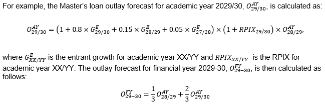
Loan outlay for each academic year is calculated using a cohort approach, based on start year and the proportion of students within each course duration. The parameters used are shown in Table 4.1, where average loan amounts are rounded to the nearest £100. The average loan amounts per year are derived from 2016/17 academic year SLC payments data. The proportions of loan recipient entrants are based on a combination of 2017/18 academic year SLC data and comparisons between the 2018-19 financial year model forecast to outturn. The expected number of loan borrowers in each cohort is multiplied by an estimated average loan amount. The estimated average loan amounts per year for a cohort are calculated by uprating the 2016/17 academic year average loan amounts by OBR outturn and forecast RPIX, from the 2017/18 academic year to the corresponding start year. The loan amount is spread across one, two or three years depending on course duration. The sum of the outlay from each cohort is aggregated to produce a final academic year outlay figure. The financial year forecast is calculated by assuming the outlay in a given financial year is equal to the sum of one third of the outlay in the first academic year it overlaps with and two thirds of the outlay in the second academic year it overlaps with.
Doctoral loans
Doctoral courses can last from 3 to 8 years. The forecast assumes the same distribution of course duration in each year of the forecast, shown below in Table 4.2. This assumption is based the distribution of course lengths in Doctoral loan application data for academic year 2018/19, with an effective date of 15th November 2018.
Table 4.2:Estimated proportion of Doctoral loan recipient entrants by course duration
Course duration
Proportion of loan recipient entrants
3 years
0.43
4 years
0.33
5 years
0.06
6 years
0.10
7/8 years
0.07
Figures may not appear to sum to 1 due to rounding.
The average loan for the whole course is estimated using a similar uprating approach to the Master’s forecast. For example, the average loan for new entrants in the 2025/26 academic year is estimated to be £ 28,968 for their whole course. This is calculated by uprating the average requested amount in 2018/19 (opens in new tab) as at end December 2018, by outturn and forecast RPIX, from the 2019/20 academic year to the corresponding start year. Note, the maximum doctoral loan amount for a course starting in 2025/26 is £ 30,301.
Annual academic year outlay is then calculated using a cohort approach based on course duration. The number of borrowers per course duration as outlined above, is multiplied by continuation rates from HESA data, to estimate the expected number of borrowers in each year for each course length. The expected number of loan borrowers in each cohort is multiplied by the corresponding average loan amount spread evenly across the course duration. The sum of the outlay from each cohort is aggregated to produce a final academic year outlay figure. Like in the Master’s loans forecast, the financial year forecast is calculated by assuming the outlay in a given financial year is equal to the sum of one third of the outlay in the first academic year it overlaps with and two thirds of the outlay in the second academic year it overlaps with.
Long-term outlay forecasts
The same methodology as documented above was used to forecast the long-term full-time and part-time undergraduate outlay, however, an alternative method was used to forecast the long-term postgraduate outlay.
Undergraduate higher education loan products
The methodology described above, used to forecast outlay for undergraduate loans was also used to produce the long-term undergraduate outlay forecast. Using individual-level data on loan borrowers provided by SLC and long-term growth rates from the entrant borrowers model, forecast students were generated for each academic year from 2025/26 to 2083/84. These students were allocated loans using forecast loan caps based on announced loan caps and the long-term OBR RPIX forecast. The loan outlay forecast was converted to a financial year forecast by apportioning loan payments made in each academic year between the financial years they straddle, according to analysis of SLC data.
Postgraduate loans
The postgraduate long-term forecast is calculated using a cohort (based on start year) approach. The growth rate for each cohort is found by taking the entrant growth from the long-term student numbers model for the academic year that the cohort started. This is then multiplied by the proportion of total borrowers from each cohort, by product, shown in Table 4.3, to give a total student loan borrower growth rate for the academic year. This student loan borrower growth rate is then multiplied by the previous academic year outlay forecast and multiplied by forecast RPIX. The financial year forecast is calculated by assuming the outlay in a given financial year is equal to the sum of one third of the outlay in the first academic year it overlaps with and two thirds of the outlay in the second academic year it overlaps with.
Table 4.3: Proportion of total borrowers by postgraduate loan product and year of study
Year of study
Proportion of total borrowers (Master’s)
Proportion of total borrowers (Doctoral)
1st year
0.80
0.40
2nd year
0.15
0.30
3rd year
0.05
0.25
4th year
−
0.05
Data quality
Student loan outlay forecasts are uncertain as they are primarily driven by borrower behaviour as well as economic factors such as inflation and household residual income. This model assumes that the characteristics and behaviour of future borrowers will be similar to historical ones derived from SLC administrative data which may not necessarily be the case. The model is also dependent on the Spring 2026 OBR macroeconomic forecasts that are used to uprate loans. Any significant changes to the economy from these forecasts could affect the outlays that will be made on student loans.
The model uses SLC administrative data to determine borrower numbers and loan amounts. The DfE receives data extracts from the Student Loans Company on an academic year basis that are used in the student loan outlay model. This data is consistent with the data published in the SLC Student Support for higher education in England publication (opens in new tab). Data on borrower sex is collected at the application stage, the only options are ‘female’ or ‘male’, and options are self-identified by loan applicants.
The model uses the growth in forecast entrants from the DfE entrant borrowers model; see Section ‘Entrant borrowers model’. The population covered includes borrowers entitled to full support that will take out either a tuition fee or a maintenance loan from Student Finance England studying at Approved (fee cap) providers but does not cover borrowers at Approved providers.
The model assumes that loans will be uprated by forecast RPIX in future years for which the maximum loan amounts have not yet been announced. With the exception of the introduction of the LLE, the model incorporates existing government policy announced by 24 April 2025 and assumes such policy will remain unchanged. Therefore, the introduction of the LLE and, if implemented by Government, any other changes to student loan eligibility, terms and conditions could affect the forecasts presented in this publication.
Table 4.4 compares the performance of the loan outlay model to SLC outturn data in 2025-26 and shows that the overall outlay forecast was approximately 1.9% lower than the outturn figure relative to the forecast. This equates to £405 million. The Undergraduate forecast was lower than the outturn with a percentage difference of -1.8% relative to the forecast. The Master’s and Doctoral forecasts were lower than the outturn with percentage differences of -3.3% and -18.7% relative to the forecast respectively.
Table 4.4: Difference between Higher Education Outlay Forecast and SLC outturn for financial year 2025-26
The DfE student loan earnings and repayments model is the financial model used to estimate the cost of income-contingent student loans to Government. It forecasts the repayments that the Department expects to receive on its expenditure on student loans.
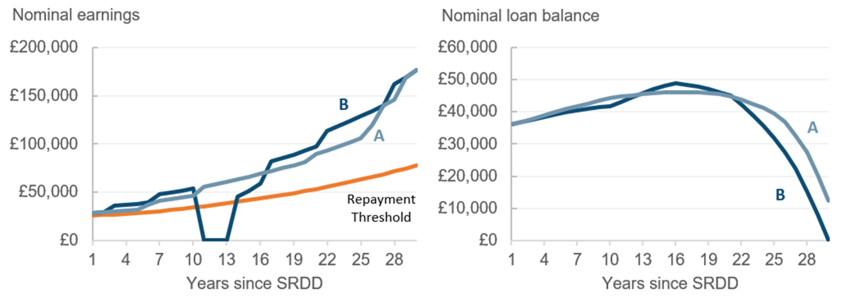
The model is a micro-simulation model. It forecasts student loan repayments by estimating future earnings for a sample of individual student loan borrowers, and applies the loan repayment policy to each borrower, before aggregating the results to estimate totals for the population as a whole. For each loan borrower, it predicts their next year’s earnings, and when this is repeated it generates an earnings path. Where historical information on earnings is available the model makes use of this. Earnings predictions are based on the borrower’s level of study, sex, years since SRDD (Statutory Repayment Due Date, typically the April following the borrower’s final point of outlay), age and other information. This allows the model to capture individual changes in earnings over the borrower’s working lifetime.
Once a borrower’s earnings have been forecast, their repayments, interest and loan balances are calculated year by year for the length of their repayment term, or until they finish repaying their loan. Further adjustments are made to some borrowers’ repayments to allow for voluntary repayments, overseas repayments, and differing obligatory repayments resulting from non-standard earnings distributions across months of the year or across multiple jobs (frictions).
The model forecasts repayments for income-contingent student loans eligible through Student Finance England. Earnings forecasts are made for undergraduates (first degrees and sub-degrees) and PGCE loan borrowers based on historical administrative data for comparable loan borrowers and historical administrative earnings data for the UK residents. For Master’s and Doctoral loan borrowers, earnings are modelled by applying a percentage uplift to an earnings forecast for a comparable first degree student.
The main data sources used in the model are:
Student Loans Company (SLC) administrative data – provides details of borrowers and the loans they take out, used to forecast earnings and employment status in early repayment years. Used for modelling migration, repayment frictions and repayments made directly to the SLC.
Longitudinal Education Outcomes (LEO) - used in earnings and employment models in early repayment years.
His Majesty’s Revenue and Customs (HMRC) administrative earnings data – used in earnings model from year 11 of repayments onwards.
Office for National Statistics (ONS) life tables – data on deaths.
ONS Average Weekly Earnings (AWE) data – used to adjust earnings between 2014-15 earnings values and nominal terms.
Student Loans Company (SLC) administrative data – used to estimate course completion rates and borrower characteristics for postgraduates, replacing HESA data which was used prior to April 2026.
Office for Budget Responsibility (OBR) macroeconomic forecasts – forecasts of earnings growth, the Bank of England base rate, RPI and RPIX published as part of their Economic and Fiscal Outlook EFOs - Office for Budget Responsibility (opens in new tab).
DfE Student numbers model – forecasts of entrant numbers.
DfE Outlay model – forecasts of student loan outlay.
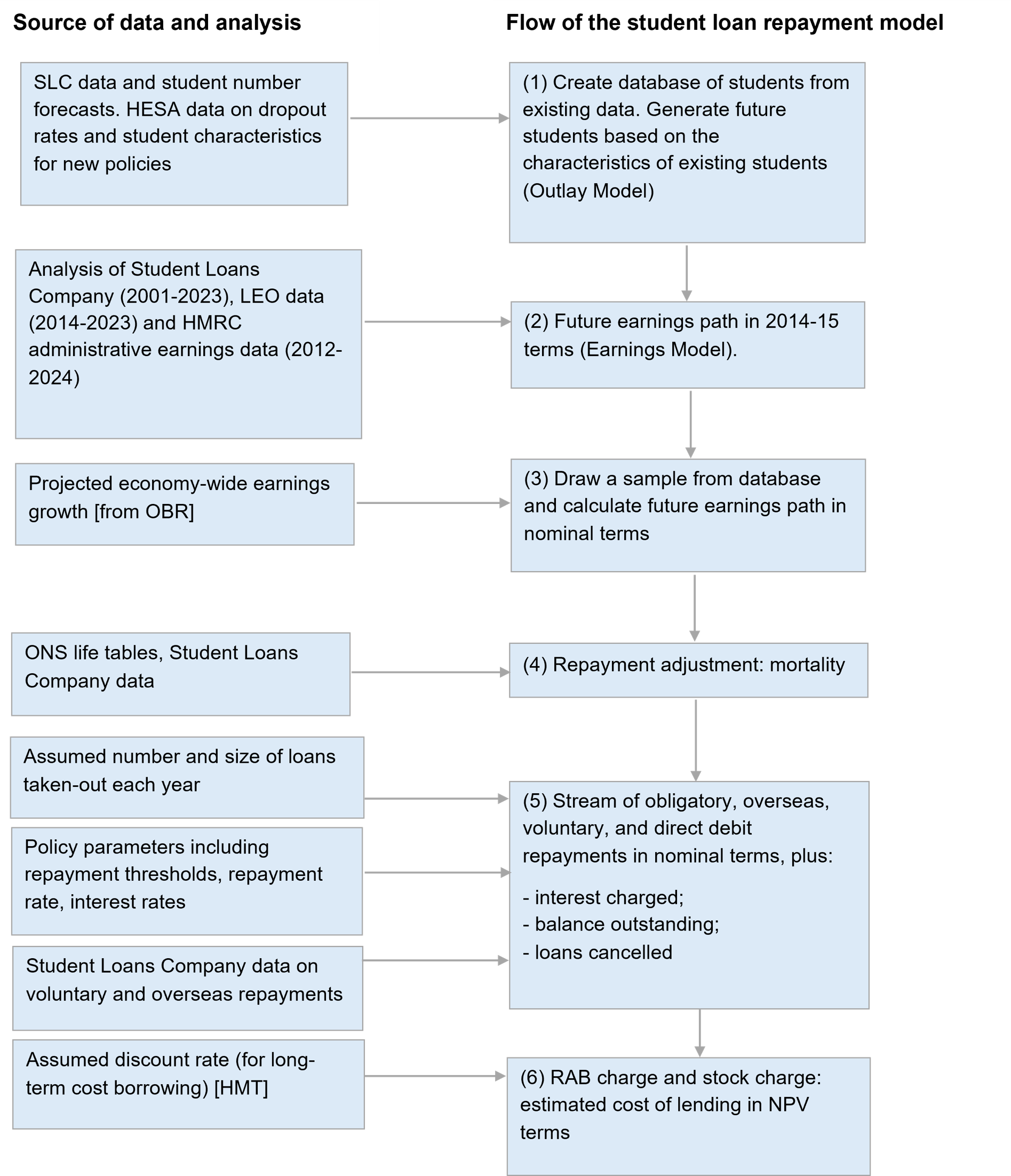
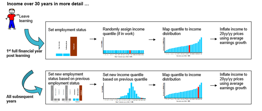
Figure 5.1: Processes and sources underlying the student loan repayment model
Figure 5.1 explains, at a high level, the processes that the model goes through to produce the forecasts, along with how each data source feeds into the full model.
Student loan repayment policies
Income Contingent Repayment (ICR) loans require borrowers to make repayments based on their annual income, starting from the April after they have left their course (the borrower’s SRDD). Under each repayment plan, borrowers are required to make repayments each tax year, through either PAYE or self-assessment, equal to a percentage of their income above a set repayment threshold until either they have fully repaid their loan balance, or their loan is cancelled. Loans are cancelled if the borrower dies, if they still have an outstanding loan balance at the end of their repayment term, or if they are in receipt of a disability related benefit and are assessed as permanently unfit for work. Loans accrue interest during and after the borrower’s course, which is added to their loan balance.
A borrower becomes liable to repay their loan on the 6th of April (start of the UK tax year) after they complete or withdraw from their course, at which point their repayment term starts on what is known as their Statutory Repayment Due Date (SRDD). There are two exceptions to this:
Part-time loan borrowers will enter repayment at the start of the tax year after four years have elapsed since the first day of the first academic year of the course, even if they are still studying.
When a loan product is first introduced, the earliest SRDD for some borrowers may be later than it would usually be. For example, all Plan 2 borrowers that completed or left their courses before April 2016 had an SRDD of April 2016, even though under the usual rule some would have had an SRDD up to three years earlier. For Plan 5 borrowers, the first possible SRDD is April 2026.
A summary of the key repayment policy details for each loan product is shown in Table 5.1 below.
Table 5.1: Key policy details for each loan product
Plan 1
Plan 2
Plan 3 (Postgraduate)
Plan 5
Earliest year of entrants
1998/99
2012/13
2016/17 (Master’s)
2018/19 (Doctorate)
2023/24
Earliest SRDD cohort
April 2000
April 2016
April 2019 (Master’s)
April 2020 (Doctorate)
April 2026
Length of repayment term
Until age 65 (entrants up to 2005/06);
25 years after SRDD (2006/07 entrants onwards)
30 years after SRDD
30 years after SRDD
40 years after SRDD
Repayment rate
9% of earnings above repayment threshold
9% of earnings above repayment threshold
6% of earnings above repayment threshold (in addition to any Plan 1, 2 or 5 repayments)
9% of earnings above repayment threshold
Interest rate
The lower of either RPI, or the Bank of England base rate +1%
RPI+3% during course, variable between RPI and RPI+3% after SRDD depending on earnings
RPI+3%
RPI
The interest rate applied to student loans is based on the Retail Price Index (RPI). The Department for Education (DfE) uses the RPI figure from the March prior to the start of the academic year to set interest rates for the following year. This ensures that the interest reflects inflation and maintains the real value of the loan over time. RPI will align with CPIH (Consumer Price Index including owner occupiers' housing costs) from 2030.
The interest rates for Plan 2, 3 and 5 student loans are subject to a Prevailing Market Rate (PMR) cap. This means borrowers will not be charged an interest rate greater than the reasonable market rate for an unsecured personal loan, with regular reviews of the cap published at Change to the Plan 2, Plan 5 and Plan 3 ('Postgraduate (PG)') student loan interest rates announcement - GOV.UK (opens in new tab). The PMR cap is currently, and is consistently forecasted as, higher than the maximum uncapped interest rate, so doesn’t currently have an effect on forecasts.
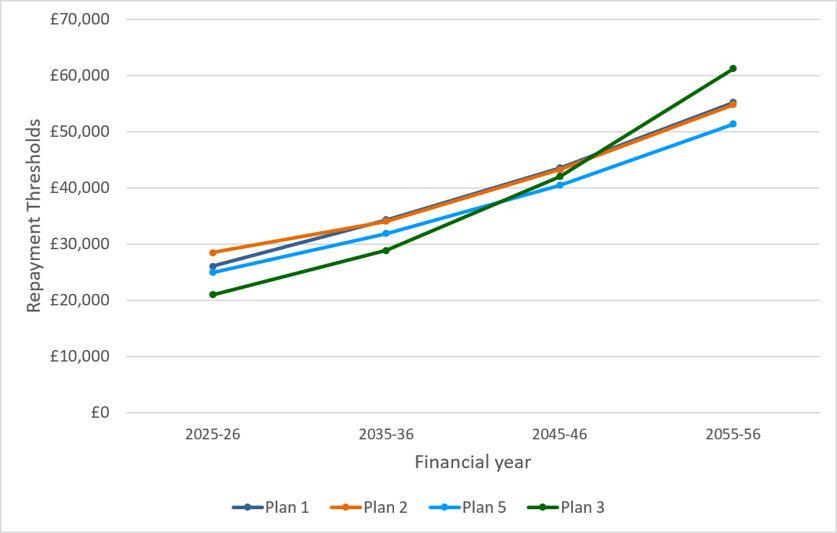
Each loan product has a separate income repayment threshold, above which repayments are made. Figure 5.2 shows the forecast repayment thresholds for each policy. All historical Plan 1, Plan 2 and Plan 3 threshold levels are published (opens in new tab), alongside Plan 4 thresholds which are applicable only to borrowers domiciled in Scotland.
The Plan 1 threshold is set at £26,065 for tax year 2025-26, and at £26,900 for tax year 2026-27. It will subsequently increase each year based on RPI.
The Plan 2 threshold was initially set at £21,000 from 2016-17 to 2017-18 before rising to £25,000 in 2018-19, to £26,575 in 2020-21, and to £27,295 in 2021-22. The threshold remained at £27,295 until the end of tax year 2024-25, after which it increased to £28,470 in line with RPI. The threshold will increase in line with RPI to £29,385 for tax year 2026-27 and will remain at this level until the end of tax year 2029-30. This is following the announcement at the 2025 Autumn budget to freeze the Plan 2 repayment threshold for 3 years from 2026-27. The Plan 3 repayment threshold is currently £21,000.
The initial Plan 5 repayment threshold is set at £25,000 until April 2027, at which point it will increase in line with RPI.
If a borrower has loans under multiple undergraduate plan types, they repay in line with the rules outlined at Repaying your student loan: How much you repay - GOV.UK (www.gov.uk) (opens in new tab). For example, if a borrower holds both a Plan 1 and a Plan 2 loan, they pay back 9% of income over the Plan 1 threshold. If their income is under the Plan 2 threshold, repayments only go towards the Plan 1 loan. If income is over the Plan 2 threshold, repayments will be split between both loans, with repayments on income between the thresholds going to the Plan 1 balance and income above the Plan 2 threshold going towards the Plan 2 balance.
Rules for borrowers with Plan 1/2 and Plan 5 loans are analogous to those with both Plan 1 and 2 loans.
Thestudent loan undergraduate repayment model forecasts future repayment thresholds for all undergraduate plan types using OBR forecasts for RPI, in line with legislation (opens in new tab).
Borrowers with a Plan 3 (postgraduate) loan repay this in parallel with any undergraduate loans (i.e. Plan 1, Plan 2 or Plan 5). Plan 3 repayments are calculated separately at 6% of income over the postgraduate threshold (£21,000 as of 2026) and are made in addition to the 9% repayment on income over the relevant undergraduate threshold(s). This means a borrower with both Plan 2 and Plan 3 loans could repay a total of 15% of their income above the respective thresholds.
To enable future repayments to be forecast, for modelling purposes it is assumed that from 2026-27 the Plan 3 loan will rise in line with Office for National Statistics (ONS) average earnings growth statistics; there is no set policy for increases to the Plan 3 repayment threshold.
Figure 5.2: Forecast repayment thresholds for each loan product
England, financial years 2025-26 to 2055-56
In addition to the repayment threshold, Plan 2 also has two interest thresholds. Once Plan 2 borrowers are past their SRDD, their interest rate varies depending on income. If their income is below or equal to the lower interest threshold their interest rate is equal to RPI; at or above the upper interest threshold it is RPI+3%; and for anyone with an income in between it varies linearly between the two.
The interest rate for Plan 2 and Plan 3 will be capped at 6% for the 2026/27 academic year Interest rate cap introduced to protect Plan 2 borrowers - GOV.UK (opens in new tab). The lower interest threshold is the same as the repayment threshold, while the upper interest threshold was set to £41,000 in 2016-17 before increasing to £45,000 in 2018-19, and £49,130 in 2021-22. It remained at £49,130 until the end of tax year 2024-25 after which it increased to £51,245 in line with RPI.
Student loan borrowers resident in the UK generally make their loan repayments through the tax system to His Majesty's Revenue and Customs (HMRC), either in-year through their employer via Pay As You Earn (PAYE) or the following year via a Self-Assessment tax return. Borrowers residing overseas are required to contact the Student Loans Company (SLC) and arrange to make repayments directly to them. Borrowers can also choose to make early repayments on their loan, directly to SLC ('voluntary repayments'). When a borrower is close to fully repaying their loan, SLC will alert them and, to avoid over-repaying via the tax system, they can arrange to make their repayments via direct debit directly to SLC rather than through HMRC.
Methodology
Loan borrower population
A population of past and future loan borrowers is created containing information about borrowers’ loan amounts, their courses, and various other information about them. To forecast a borrower’s earnings the model needs data on their characteristics such as:
Higher Education provider group (see list of higher education provider groups below)
1994 Group: Loughborough, East Anglia, Leicester, Lancaster, Sussex, Essex, Goldsmiths, Royal Holloway, IoE, SOAS, Birkbeck
University Alliance: Manchester Metropolitan, Sheffield Hallam, Nottingham Trent, UWE, Liverpool John Moores, Northumbria, Plymouth, De Montfort, Portsmouth, Kingston, Hertfordshire
MillionPlus: Leeds Metropolitan, Central Lancashire, Wolverhampton, Middlesex, Birmingham City, London Metropolitan, East London, Staffordshire, Derby, Sunderland
GuildHE: Southampton Solent, Worcester, York St John, Winchester, Chichester and many arts university colleges
Large non-affiliated: Brighton, Hull, Westminster, Kent, Edge Hill, Brunel, Strathclyde, Reading, Swansea, Roehampton, Gloucestershire, Bath, Heriot-Watt
Small non-affiliated: Numerous small colleges
Course subject classifications, with typical subjects of study, are as follows:
Medicine and Dentistry: Medicine, Dentistry (both pre-clinical and clinical)
Subjects allied to Medicine: Anatomy, Pharmacy, therapies, nutrition, optometry, audiology, nursing, medical technology, environmental health
Biological Sciences: Anatomy, Pharmacy, therapies, nutrition, optometry, audiology, nursing, medical technology, environmental health
Veterinary Sciences, Agriculture: Veterinary Medicine and Dentistry (both pre-clinical and clinical), animal science, agriculture, forestry, food studies
Architecture, Building & Planning: Architecture, Surveying, Building, Landscape design, Planning
Social Studies: Economics, Politics, Sociology, Social Policy, Social Work, Anthropology, Human geography, Development studies
Law: Law by area, law by topic
Business & Administrative Studies: Business Studies, Management, Finance, Accounting, Marketing, HR management, office skills, hospitality/tourism
Mass Communication and Documentation: Information Services, public relations, Media studies, Publishing, Journalism
Linguistics and Classics: Linguistics, Literature, English studies, Ancient language studies, Celtic studies, Latin studies, Classical Greek studies, Classics
European Languages and Literature: French studies, German studies, Italian studies, Spanish studies, Portuguese studies, Scandinavian studies, Russian and East European Studies, European Studies
Other Languages and Literature: Chinese studies, Japanese studies, South Asian studies, Asian studies, African studies, Modern Middle Eastern studies, American studies, Australasian studies
Historical and Philosophical Studies: History by period, History by area, History by topic, Archaeology, Philosophy, Theology and religious studies, Heritage studies
Creative Arts and Design: Fine art, Design studies, Music, Drama, Dance, Cinematics and photography, Crafts, Imaginative writing
Education: Teacher training, research and study skills in education, academic studies in education
Combined courses and others not coded: Combined or unknown subject area
Earnings forecasts
The part of the student loan earnings and repayment model that forecasts earnings is known as the earnings model. The earnings model predicts earnings for each individual for up to 43 years past their SRDD, by which point any outstanding loan balances will have been written off.
An estimate of the earnings path of loan borrowers is necessary to estimate a borrower’s repayments across their repayment term. As loans generate interest throughout their repayment period, the path of an individual’s earnings, rather than their total earnings over the repayment period, has a significant effect on the amount of the loan the borrower will repay.
Figure 5.3 depicts two hypothetical earnings scenarios, A and B, for a Plan 2 loan borrower with the same SRDD and the same nominal loan balance at their SRDD of c. £35,000. In both cases the individual has the same total nominal earnings over their supposed 30-year repayment period (for Plan 2 loans); however, in scenario B the loan is completely repaid, whereas in scenario A part of the loan (c. £12,000 nominal loan balance) is written off.
Figure 5.3: Earning and loan balance paths for a hypothetical loan borrower with earnings scenarios A and B
The earnings model is divided into two parts, based on the number of years between the forecast year and a borrower’s SRDD. The first 10 years after SRDD are predicted using the ‘early-career earnings model’ and years 11 to 43 are predicted using the ‘long-term earnings model’. The models are split in this way due to different data availability for these periods.
Forecasts are produced based on the assumption that future earnings will follow the same trajectories as those seen in recent historical earnings. In the early-career model these historical earnings are derived from two sources:
Student Loans Company (SLC) administrative data from 2001 to 2023
Longitudinal Education Outcomes (LEO) data from 2014 to 2023
The SLC data includes earnings and employment status in each tax year following a borrower’s SRDD as well as characteristics of the borrower’s most recent period of study, such as subject of study, provider and course level. SLC data does not, however, include the earnings of those who have fully repaid their loan and therefore, once high earners start to repay their loans in full, the dataset provides an unbalanced picture of the earnings of the graduate population. To overcome this, where borrowers have repaid their loans, earnings are taken from the LEO dataset where available, based on fuzzy matching between the SLC and LEO datasets. The model is trained on a subset of the data, from 2014 to 2023, containing earnings and characteristics for borrowers up to 10 years after SRDD.
In the long-term earnings model, historical earnings are derived from HMRC administrative earnings data for 10% of the UK population from 2012 to 2024. This data includes a person’s age and gender (provided as “female” and “male” options), as well as their PAYE and self-assessed earnings. It is not possible to distinguish whether or not people in this dataset are graduates or not. Therefore, it would not be suitable for predicting earnings earlier in a graduate’s career, where we expect a degree qualification to have a signalling effect resulting in graduates earning more on average than non-graduates, even once sex, age and earnings history are taken into account. By 11 or more years after SRDD we assume the label of graduate or non-graduate is immaterial, as any signalling effect is already encompassed within individual’s earnings history (given age and sex. Therefore, the HMRC data offers a richer source of data on earnings for people later in their careers, compared to the SLC/LEO datasets. The Average Weekly Earnings (AWE) index, published by the ONS, is used to re-baseline historical earnings into 2014-15 financial year terms, allowing us to make predictions based on the full-time-series of earnings, having already accounted for wage inflation between years.
To create an earnings path for each borrower, both models search their respective training datasets to find the 10 most similar individuals based on various characteristics. In the early-career model, similar individuals are selected from the population with the same number of years since SRDD. The variables that define the proximity between individuals are their Higher Education Institute type, domicile (England or “Borrowers granted partial higher education support under the regulations”), subject of study, sex, age, whether or not the borrower withdrew from studies before graduation and up to three years of previous PAYE and self-assessed earnings. In the long-term model, individuals are selected from the population with the same age and sex, and the previous three years of PAYE and self-assessed earnings are used to define proximity. This proximity is measured by Euclidean distance.
To produce an earnings forecast, the model then selects one of those individual’s known earnings in the following year, choosing the individual based on a weighted probability, where weights are the square inverse of the Euclidean distance. Where the weights of the 10 selected individuals are identical, the model selects one at random. Annual PAYE and self-assessed earnings are forecast for each borrower in the sample, and this step is repeated over subsequent years, to generate an earnings path for each individual. Forecasts are produced in 2014-15 financial year terms, and later re-scaled using OBR earnings growth forecasts.
Whilst undertaking a course we do not forecast earnings for borrowers. This includes part-time loan borrowers studying for longer than 4 years who have an SRDD in the fifth April after the start of their course, even if they are still studying. Similarly, we do not account for the impact of earnings prior to taking up a university course on earnings on completion. As such, estimated earnings for part-time loan borrowers may be lower than actuals on entry into the labour market. However, we do not expect this impact to be long lasting and modelled earnings for part-time loan borrowers will tend towards those of full-time loan borrowers as they progress through their career.
Mortality
ICR loans can be cancelled prior to the end of the repayment term if the borrower dies. The probability of death in a given year is derived, based on the borrower’s age and sex, from ONS life tables and SLC data. SLC data shows lower write-off levels than would be expected from ONS mortality rates, most likely reflecting that graduates have lower mortality rates than non-graduates of the same age. However, the historical SLC data has little coverage of student loan borrowers aged above their mid-30s, so a weighted average of the two sets of mortality rates is taken that gives a high weighting to the SLC data at younger ages and to ONS data at older ages.
There are reasons other than death why a loan may be written off before the end of a borrower’s repayment term such as being assessed as permanently unable to work; however, the level of these write-offs is comparatively small and as such they are not included in the model. There is also a risk that including such write offs explicitly may lead to double counting – such borrowers will still be present in the HMRC data used to train the earnings model, appearing as individuals with £0 earnings, so they are already implicitly included in the model, just with write-off occurring later (at the end of the repayment term). Timing of write-offs is irrelevant to most metrics – timing of repayments is what matters most to the RAB charge. Whether written off sooner or later, repayments remain £0 beyond that point.
Repeat borrowers and periods of study (POSs)
In calculating the Doctoral RAB (Resource Accounting and Budgeting) charge, we assume that some borrowers will already have Plan 3 loans from their Master's courses. The RAB charge for Doctoral loans is calculated as a marginal RAB, focusing on the additional borrowing specifically for the Doctoral loan. This ensures that the entire additional subsidy generated by taking a Doctoral loan is accounted for as part of the Doctoral cost.
This approach contrasts with undergraduate borrowing, where an additional period of study increases the borrower's total loan amount. This makes repaying the existing loan balance more difficult and effectively increases the RAB charge for the earlier loan. This behaviour is included in the forecast and the increased RAB for past loans is accounted for.
Repayments made directly to SLC
In addition to obligatory repayments collected through the UK tax system, repayments can also be paid directly to the SLC. These fall into three main categories:
Voluntary repayments – These are (early) repayments made by the individual in addition to their obligatory repayments.
Payments from overseas – Repayments from borrowers situated overseas cannot be collected through the tax system. Overseas borrowers make obligatory repayments directly to the SLC based on their income and the earnings threshold Overseas earnings thresholds for Plan 2 student loans - GOV.UK (opens in new tab) for their country of residence.
Direct debits – In the last couple of years of payment the SLC offer the borrower the opportunity to repay the rest of their loan through a direct debit to prevent overpayment.
The probability of a borrower making a voluntary repayment each year is generated from a multinomial logistic regression model based on SLC administrative data. Voluntary repayments are particularly dependent on the magnitude of the debt outstanding and the number of years into the repayment period, as well as whether a borrower has previously made a voluntary repayment. The regression model also takes into account obligatory repayments, whether a borrower is close to repaying their loans in full, earnings and the proportion of the balance previously paid via voluntary repayments. Most voluntary repayments come from borrowers with low amounts of debt in the first few years of repayment.
If a borrower is due to make a voluntary repayment in the model, they are either categorised as repaying their outstanding balance in full or repaying a percentage of the debt outstanding as a direct repayment. For those borrowers not repaying their outstanding balance in full, the percentage to be repaid is derived using a second logistic regression model. This model takes into account voluntary repayments in prior years, the number of years into the repayment period, outstanding balance, earnings, and obligatory repayments.
Borrowers can also make overseas repayments. The probability of a borrower making an overseas repayment each year is generated from a decision tree model based on SLC administrative data. The decision tree model considers the borrower’s plan type, earnings over the threshold, and previous overseas repayments. The size of the repayment is selected at random from a distribution of repayment amounts based on the borrower’s overseas repayments last year and their plan types.
Postgraduate loan borrowers
Limited historical data on postgraduate loan borrowers is available as they are relatively new loan products (introduced in 2016). In addition, information on postgraduate earnings and behaviours from survey data is limited, as in population surveys the proportion of the survey respondents that have postgraduate degrees is very small. Therefore, the student loan repayment model generates employment and earnings forecasts for postgraduate loan borrowers using the same earnings model as for first degree students with the same characteristics, to which it then applies a fixed uplift to earnings in all years to account for the higher earnings postgraduates are expected to have.
For Master’s borrowers an earnings uplift of 8.9% is applied for male borrowers and 10.3% for female borrowers. This is based on research that estimated this to be the average marginal earnings gain for Master’s students on top of their undergraduate degree (Conlon & Patrignani, 2011). For Doctoral students, an earnings uplift of 8.0% is applied for male borrowers and 6.0% for female borrowers. These uplifts are based on results for Doctoral students from the same research, though they have been adjusted down to account for trends associated with the subject of study and HEI group. This adjustment aims to account for factors such as these, which were not considered directly in the research due to the available sample size but are important in student finance forecasting. For example, the population of students expected to take up Doctoral loans is not representative of all Doctoral students since the availability of other funding sources (such as industry or research council funding) may differ by the subject of study. These uplifts for Master’s and Doctoral students are not directly comparable, as other factors will also affect the average earnings for each course level.
The Doctoral RAB charge accounts for existing Master’s Plan 3 borrowing by considering the proportion of doctoral loan borrowers who also have Master’s loans. This means the RAB charge for doctoral loans includes the expected non-repayment of both Doctoral and Master’s loans when calculating the overall subsidy.
Essentially, it integrates the repayment forecasts for both types of loans and discounts them back to the period the loans were issued, using a specific discount rate. This ensures that the government's subsidy to the student loan system accurately reflects the combined financial impact of both Doctoral and Master’s Plan 3 loans.
As there is only very limited administrative information available, postgraduate loan borrowers are assumed to have similar post-study behaviours as an equivalent first degree student for factors such as voluntary repayments, overseas repayments and mortality.
Obligatory repayment amounts
Once annual earnings are calculated and non-employment, migration, and mortality are taken into account, the obligatory repayments are calculated according to the deterministic repayment rules for that year. Once obligatory repayments have been calculated, a repayment frictions model is applied to them to reflect the historical differences observed between repayments due based on the deterministic calculation and observed obligatory repayments. These frictions can be due to factors such as seasonal earnings patterns (which could result in higher repayments than otherwise) or the borrower’s earnings coming from multiple jobs (which could result in lower repayments than otherwise).
Repayment frictions
The probability of a borrower having a repayment friction each year is generated from a decision tree model based on SLC administrative data. Incidence of repayment frictions are dependent on the magnitude of the debt outstanding for loans of various plan types, earnings in both the current and prior year, the change in earnings, the number of years into the repayment period, as well as a borrower’s repayment frictions in the prior year.
If a borrower is due to have a repayment friction in the model, they are either categorised as having a positive friction (borrower repaying more than they are obliged to based on earnings), a large negative friction (borrower repaying less than they are obliged to based on earnings), or a small negative friction (less than £15).
For those borrowers due to have a small negative friction, the repayment adjustment is taken from a random distribution of historical small negative repayment frictions. For borrowers due to have a positive friction, the repayment adjustment is selected at random from a distribution of repayment amounts (expressed as percentages of earnings over the repayment threshold) based on the borrower’s plan types, earnings over the threshold and earnings change from the prior year.
Finally, for borrowers due to have a large negative friction, a multiple regression model is used to determine the size of the repayment friction. This model uses a borrower’s frictions in the prior year, earnings change from the prior year, obligatory repayments in the prior year, and obligatory repayments in the current year.
Repayment amounts and debt outstanding
All obligatory, voluntary, and overseas repayments that the borrower makes each year are summed together, up to a maximum of the borrower’s remaining loan balance. Borrowers are assumed to stop repaying their loan once their loan balance reaches zero. The model does not account for borrowers making overpayments or receiving refunds after overpaying.
To calculate the size of a borrower’s loan balance, borrowers are given annual outlay amounts while on their course based on the distribution of outlay amounts of historical borrowers in the SLC data, uprated in line with forecast RPIX depending on the appropriate loan policy. Capitalised interest is accumulated and added to the borrower’s balance each year, with any repayments subtracted from it. The size of the borrower’s debt is calculated on this basis each year until they either fully repay their loan or until their loan is cancelled, either due to mortality or because they reached the end of their repayment term.
In reality, HMRC share repayment data with SLC on a weekly basis, but as an approximation all PAYE and voluntary repayments in the model are assumed to be made in the middle of the financial year. Repayments from self-assessment (SA) are correctly assumed to be made at the end of each January, for income in the previous financial year. Interest for the first half of the financial year is added to the debt outstanding at the start of the year before PAYE and voluntary repayments are made, then the interest for the next four months is added after they have been deducted, then finally the interest for the final 2 months is added after any SA repayments have been deducted.
In academic years where a borrower is forecast to receive loan outlay, payments are assumed to occur in three instalments at the end of September, January and April. Interest is accrued on these payments and applied to the loan balance accordingly.
If a borrower’s loan is cancelled this is assumed to happen at the end of the financial year, as this is the point when cancellations will occur at the end of a borrower’s repayment term, which accounting for the large majority of cancellations across the loan book.
Interest rates each year are calculated from RPI, the Bank of England base rate (Plan 1 only) and borrowers’ income in line with the appropriate policy. Additionally for Plan 2, 3 and 5, where RPI would mean an interest rate is greater than the typical rate for an unsecured personal loan, the interest rate is capped at the prevailing market rate. Regular reviews of the cap published at Change to the Plan 2, Plan 5 and Plan 3 ('Postgraduate (PG)') student loan interest rates announcement - GOV.UK (opens in new tab). Plan 2 and Plan 3 interest rates are capped at 6% in line with announced policy.
Future RPI and Bank of England base rate figures are based on OBR forecasts. The interest rates for each part of the year are calculated and then combined into an annual average that is used across the financial year. For all loan plans, the RPI figure used in calculating interest rates changes each September to the March RPI figure published by ONS in the same year (relating to the 12 months up to end of March that year), but as OBR only publishes quarterly forecasts (and in the long run only annual forecasts) the model uses the forecast for the equivalent January to March quarter in the short run, and the annual figure for the same financial year in the long run. For Plan 1 loans, quarterly base rate forecasts are averaged over each financial year, with this average +1% compared to the financial year RPI to determine which to use for interest rates that financial year.
Population totals
Forecasts for individual loans are aggregated together to estimate totals for the whole student loan population. Rather than making estimates for the whole population of loans, to make the model more resource efficient, forecasts use a sample of loans, with weightings applied to these loan results to ‘scale up’ to the correct totals for the whole population.
For the undergraduate forecast, a stratified sample of approximately 500,000 borrowers is used, covering entrants from academic years 1998/99 to 2044/45 (excluding those that have already finished repaying their loans or had them cancelled).The long-term undergraduate forecast’s stratified sample covers entrants for a longer period from 1998/99 to 2083/84 (excluding those that have already finished repaying their loans or had them cancelled). The sample is stratified by a range of loan and borrower characteristics. Loans are then randomly sampled within these strata. This stratified approach ensures that the mixture of loans in the sample remains relatively consistent from year to year.
The postgraduate model draws a representative random sample from a single entrance cohort, which is then replicated and scaled to represent each subsequent year of postgraduate entrants.
As the Doctoral loan was introduced in academic year 2018/19, limited historical outlay data were initially available. As a result, Doctoral borrowers were previously modelled using historical HESA data. This has now been updated, and the Doctoral loan model uses SLC administrative data from 2023, which are representative of real Doctoral borrowers. A fixed sample size of Doctoral borrowers is retained, with results scaled to match forecast entrant numbers.
The scaling used to increase the sample results to population totals is weighted based on several variables to reduce the sampling bias in the model. The variables used in the weighting are course start year, SRDD, sex, course level, whether the course is a STEM subject, plan type, whether the loan is for full-time or part-time study, and how many loans the borrower has.
The Resource Accounting and Budgeting (RAB) charge and the stock charge
The RAB and stock charges are the estimated cost to Government of providing a subsidy for the student finance system. They are the proportion of loan outlay (the RAB charge) and of the total outstanding loan balances (the stock charge) that are expected to not be repaid when future repayments are valued in present terms.
To calculate the RAB charge, the total outlay in a given year is added up and compared to the total net present value (NPV) of the repayments that are anticipated in connection with this same outlay. The RAB charge is calculated as
Similarly, the stock charge is calculated by summing all outstanding loan balances at the start of the year and comparing this to the total net present value (NPV) of the repayments that are anticipated in connection with these loans. The stock charge is calculated as
The NPV of future repayments is calculated by discounting all future repayments at a rate of RPI-0.55% per year until the end of the financial year 2029-30, and RPI+0.35% per year from the financial year 2030-31, to the same point in time as the loan outlay or loan balance. This is the discount rate for financial instruments set by HM Treasury (HMT) (opens in new tab) and is intended to reflect the cost of Government borrowing. The step change in 2030 reflects the alignment of RPI methodology with CPIH.
Student loans are valued in DfE’s annual accounts in line with the International Financial Reporting Standard (IFRS) 9, under which where future cash flows are discounted to measure the fair value of a financial asset. This should be done using the higher of the rate intrinsic to the financial instrument or the His Majesty's Treasury (HMT) discount rate. For student loans the intrinsic rate would be the discount rate that gave a RAB or stock charge of 0%, so the HMT discount rate is used provided the RAB charge is greater than 0%. Should the HMT discount rate result in a RAB charge calculation giving a negative value then the intrinsic rate is used instead, meaning that that RAB charge will take a value of 0%.
In the model, RAB charges are calculated for the loan book as a whole by first calculating the NPV of repayments against individual loans, then for each year aggregating these together across all borrowers and comparing them to their total loan outlay in that year. Stock charges are calculated in the same way, aggregating the NPV of individuals’ repayments before aggregating them to a population total and comparing this to the face value of the loans at that point in time.
Where a borrower has more than one year of outlay or has both future loan outlay and an existing loan balance that will be included in the stock charge, future repayments are allocated between each year of their loan outlay and their existing loan balance in proportion to the relative balances of each loan when valued at the same point in time (i.e. taking into account interest accrued on the earlier loan balances). A RAB charge is no longer produced for Plan 1 loans as very few Plan 1 students are still receiving loans.
Plan 2 loan RAB charges for both undergraduates and ALLs become less reliable over time because the last new Plan 2 borrowers started their course in academic year 2022/23, so fewer students receive Plan 2 outlay and over time they become less “typical” – a Plan 2 borrower in 2026/27 will be in their fifth year since receiving their first outlay.
Data quality and sensitivity analysis
RAB and stock charge estimates require earnings, inflation and repayments forecasts covering the subsequent 40 years. These forecasts depend heavily on input data sources, modelling techniques and assumptions used in the model. Consequently, forecasts are inherently uncertain owing to the inevitable uncertainties associated with these sources, assumptions, and methods. For example, the model assumes that the distribution of future earnings paths will be similar to historical distributions derived from SLC and HMRC administrative data, which will not necessarily be the case, particularly in the long term.
The model is dependent on the OBR macroeconomic forecasts that it uses to uprate earnings, calculate interest rates and repayment thresholds, and to discount future repayments to present values. Any significant changes to the economy from these forecasts could affect the repayments that will be made on student loans.
'Where future cash flows are discounted to measure fair value, entities should use the higher of the rate intrinsic to the financial instrument and the real financial instrument discount rate set by HM Treasury (promulgated in Public Expenditure System (PES) papers) as applied to the flows expressed in current prices.'
For the purpose of valuing student loan repayments, when the discount rate falls the value of future repayments goes up, and vice versa.
Table 5.2 shows that when the discount rate (by 0.2ppt) and the earnings growth rate (by 1ppt) are both increased, the RAB charges for undergraduate borrowing falls for all plan types. Increased earnings growth pushes more borrowers above the repayment threshold, leading to higher repayments and a reduced government subsidy. Although the higher discount rate lowers the present value of future repayments, this effect is outweighed by the stronger earnings growth.
For Plan 5, the RAB charge falls by 2 percentage points in this scenario. The impact of increased earnings growth is more limited than observed for Plan 2 – a higher proportion of Plan 5 borrowers are expected to fully repay already so increased earnings have less of an effect across the population. Furthermore, since Plan 5 borrowers are not expected to repay significantly more than they borrowed, the effect of the discount rate change is also less pronounced.
The opposite is seen when the discount rate and earnings growth are both reduced, with all RAB charges being elevated, driven by lower future earnings.
The sensitivity to earnings growth and the discount rate can also be seen in the table, showing opposite effects from the two sensitivities, with the discount rate having a far smaller impact.
When the discount rate is increased and average earnings reduced, we see a higher RAB charge, reflecting the reduction in average earnings. Similarly, when the discount rate is decreased and earnings growth increase, we see a lower RAB charge thanks to increased earnings leading to higher future repayments.
We test the sensitivity around RPI and RPIX together – inflation measures are likely to move together. RPIX is a key -term assumption in forecasting fee and maintenance loan outlay. RPI is used to set interest rates, repayment threshold uplifts and in calculating the absolute discount rate. From Feb 2030, RPIX is aligned with CPI and RPI aligned with CPIH.
Varying RPI has a large effect on RABs and stock charges. For all plans, increasing RPI raises interest rates and therefore the face value of future loan balances. Increased RPI also leads to higher repayment thresholds, meaning a borrower with the same salary will repay less per year. Furthermore, higher RPI means a higher absolute discount rate, reducing the present value of future cashflows. With no change to the earnings growth rate, fewer borrowers in the model fully repay their loans, driving up both the stock charge for Plan 1 loans and the RAB charges for Plan 2 and Plan 5 loans. Increasing the RPI uplift from 1pp to 2pp shows that this relationship is not strictly linear, although in this case the changes to stock and RAB charges approximately double. When the RPI forecast is flexed downwards the opposite happens, lowering both the stock and RAB charges. However, RAB charges for Plan 2 and Plan 5 loans do not fall by the same amount as they rose when RPI was increased, reinforcing the nonlinear relationship between RPI and RAB.
Table 5.2a: Sensitivity of Stock and RAB charge forecasts to variations of key economic inputs
Macroeconomic change
Plan 1 stock charge
Plan 2 full-time RAB charge
Plan 2 part-time RAB charge
Plan 5 full-time RAB charge
Plan 5 part-time RAB charge
HMT discount rate +0.2pp, earnings growth +1.0pp, until 2031
-2pp
-4pp
-3pp
-2pp
-2pp
HMT discount rate +0.2pp, earnings growth -1.0pp, until 2031
+3pp
+5pp
+5pp
+3pp
+3pp
HMT discount rate -0.2pp, earnings growth +1.0pp, until 2031
-3pp
-5pp
-4pp
-3pp
-3pp
HMT discount rate -0.2pp, earnings growth -1.0pp, until 2031
+2pp
+4pp
+4pp
+2pp
+2pp
RPI & RPIX +1.0pp throughout the forecast period
+4pp
+ 11pp
+11pp
+11pp
+10pp
RPI & RPIX +2.0pp throughout the forecast period
+7pp
+ 20pp
+20pp
+22pp
+19pp
RPI & RPIX -1.0pp throughout the forecast period
-1pp
-11pp
-10pp
-9pp
-8pp
RPI & RPIX -2.0pp throughout the forecast period
-5pp
-22pp
-19pp
-17pp
-15pp
Earnings growth +1.0pp until 2031
-3pp
-4pp
-3pp
-3pp
-2pp
Earnings growth –1.0pp until 2031
+3pp
+4pp
+4pp
+3pp
+3pp
HMT discount rate +0.2pp until 2031
0pp
+1pp
+1pp
+1pp
+1pp
HMT discount rate –0.2pp until 2031
0pp
-1pp
-1pp
-1pp
-1pp
Table 5.2b: Sensitivity of Stock and RAB charge forecasts to variations of key economic inputs for ALL
Macroeconomic change
Plan 2(ALL) RAB charge
Plan 5(ALL) RAB charge
HMT discount rate +0.2pp, earnings growth +1.0pp, until 2031
-3pp
-2pp
HMT discount rate +0.2pp, earnings growth -1.0pp, until 2031
+7pp
+3pp
HMT discount rate -0.2pp, earnings growth +1.0pp, until 2031
-5pp
-3pp
HMT discount rate -0.2pp, earnings growth -1.0pp, until 2031
+6pp
+2pp
RPI & RPIX +1.0pp throughout the forecast period
+20pp
+10pp
RPI & RPIX +2.0pp throughout the forecast period
+37pp
+18pp
RPI & RPIX -1.0pp throughout the forecast period
-13pp
-8pp
RPI & RPIX -2.0pp throughout the forecast period
-21pp
-14pp
Earnings growth +1.0pp until 2031
-4pp
-3pp
Earnings growth –1.0pp until 2031
+6pp
+2pp
HMT discount rate +0.2pp until 2031
+1pp
0pp
HMT discount rate –0.2pp until 2031
-1pp
-1pp
Table 5.2a&b shows the percentage point (pp) change to the forecast 2025-26 stock (Plan 1 loans) and RAB (Plan 2 and Plan 5 loans) charges as a consequence of varying each listed macroeconomic input up or down by 1pp or 2pp from years where there are no published outturn values. For discount rate and earnings growth rate, changes were varied up to 2030-31, RPI was varied for the length of the forecast from 2025-26 onwards. RPIX is varied alongside RPI.
Table 5.3a: Sensitivity of RAB charge (Undergraduate) forecasts to variations of key policy inputs
Policy change
Plan 1 Stock charge
Plan 2 full-time RAB charge
Plan 2 part-time RAB charge
Plan 5 full-time RAB charge
Repayment threshold
+£1,000
+2pp
+1pp
+1pp
+1pp
-£1,000
-1pp
-2pp
-1pp
-1pp
Table 5.3b: Sensitivity of RAB charge(Advanced learner loans) forecasts to variations of key policy inputs
Policy change
Plan 2 (ALL) RAB charge
Plan 5 (ALL) RAB charge
Repayment threshold
+£1,000
+1pp
+2pp
-£1,000
-2pp
-2pp
Table 5.3a&b shows the percentage point (pp) changes to the forecast 2025-26 RAB charges as a consequence of varying the repayment threshold by £1,000 in 2025-26 (with the threshold growing at the usual rate after that depending on policy for the loan type).
The model uses SLC administrative data to determine borrower characteristics, loan amounts, earnings in the first three years of their repayment term and repayments made directly to SLC. As an administrative source, the historical SLC data should be broadly accurate, although forecasted earnings and direct repayment forecasts rely on future borrowers having similar behaviours to historical borrowers.
Where new loan products have been introduced, the forecasts are more uncertain as there is less historical information available on which to base forecasts and more uncertainty about what student behaviours will be in response to policy. This is particularly the case for the two postgraduate loan products, for which the earnings forecasts are less well developed than for undergraduates and for which there is very limited historical information about loan borrowers’ characteristics and behaviours. We would expect a borrower taking a loan for postgraduate study to have different characteristics to a borrower funded through other means, such as research council funding, so population level data for postgraduate students are not representative of borrowers.
Since the 2025 publication there have been a number of updates to the forecast. There have been revisions and updates to input data, economic assumptions, policies and modelling methodology. These have all combined to change the forecast RAB charges for 2025-26 in comparison to the previous publication. The effect of these factors on the RAB forecast is shown in Table 5.4. The figures are rounded to the nearest percent or percentage point.
Methodology updates: improvements and fixes to the repayments model.
Table 5.4a: Changes in the 2025-26 RAB charge for Plan 2 full-time higher education loans in comparison to the previous publication (July 2025).
25-26
26-27
27-28
28-29*
29-30*
July-2025 annual publication
34%
36%
39%
39%
0%
July-2026 annual publication
39%
43%
46%
50%
0%
Change since July 2025 publication
+5pp
+7pp
+7pp
+11pp
+0pp
Note: all figures are rounded to the nearest percentage / percentage point. The change is calculated from the raw numbers and then rounded – therefore the change may differ from subtracting the rounded components. *The Plan 2 RAB charge becomes less reliable over time due to the last new Plan 2 loans being issued in 2022/23; recipients of Plan 2 outlay in 2028-29 will be unusual.
Table 5.4b: Changes in the 2025-26 RAB charge for Plan 5 full-time higher education loans in comparison to the previous publication (July 2025).
25-26
26-27
27-28
28-29
29-30
July 2025 annual publication
30%
30%
30%
30%
30%
July-2026 annual publication
33%
34%
34%
34%
34%
Change since July 2025 publication
+3pp
+4pp
+4pp
+4pp
+4pp
Note: all figures are rounded to the nearest percentage/percentage point. The change is calculated from the raw numbers and then rounded – therefore the change presented may differ from subtracting the rounded components.
Comparison of forecast earnings with actuals
Earnings forecasts from prior years can be compared to actual earnings that subsequently become available in the SLC administrative data. One way to assess the accuracy of the forecasts is to calculate the differences (positive or negative) between forecasts and actuals for each individual borrower. Figure 5.4 shows the distribution of these individual-level absolute errors as the number of years since a borrower’s SRDD increases. Accuracy is lower in the first few years after SRDD as there is relatively little data on the previous earnings of these borrowers and improves as data on prior earnings becomes available.
Figure 5.4: The distribution of absolute differences in predicted and actual earnings for borrowers in repayment between 2022-23 and 2023-24
The individual-level errors shown in Figure 5.4 can be fairly large, for example, if the employment status of a borrower is incorrectly predicted. While minimising individual-level errors can help to predict accurate earnings trajectories, accuracy at the individual level is not necessary when calculating population-level financial metrics such as the RAB charge. Here, it is more important that the distribution of earnings is accurate, particularly around repayment thresholds. This can be assessed by comparing predicted and actual earnings distributions, as shown in Figure 5.5. Note that the assessment of the long-term model only includes years up to a maximum of 24 years after SRDD, as actual earnings are not available beyond that yet. The distribution of long-term earnings is lower than that of the early-career earnings as these are primarily Plan 1 borrowers who are yet to repay their loans and are therefore skewed towards lower earners.
Figure 5.5: Forecast and actual distributions of earnings between 2022-23 and 2023-24 for borrowers still repaying, with different numbers of years since their SRDD
The difference between predicted and actual earnings distributions can be summarised as the Wasserstein distance. When updating the model, we conduct testing to check that any changes lead to reductions in accuracy metrics such as the individual-level absolute error and the Wasserstein distance.
Comparison of forecast repayments with actuals
The student loan repayment model is designed to forecast repayments across loan borrowers’ repayment terms. Comparisons between forecast repayment totals (one or two years ahead) for individual years and the actual outturn data can give an indication of how well the model has been performing. Table 5.5 shows how recent outturn figures compare with the forecasts made at the time. Improvements are made to the student loan earnings and repayment model each year and the data used in it are updated, so forecasts are shown as made at both the start and end of each tax year. The financial year 22-23 forecast might be less accurate due to COVID effects, and we are still investigating this.
Table 5.5: Forecast and outturn repayments across all higher education loan products
Outturn
Forecast
Tax Year
Date
£ million
Date
£ million
Difference
2013-14
30/04/2014
1,590
31/03/2014
1,630
2.5%
2014-15
30/04/2015
1,750
31/03/2014
1,870
6.9%
31/03/2015
1,920
9.7%
2015-16
30/04/2016
1,930
31/03/2015
2,140
10.9%
31/03/2016
1,930
0.0%
2016-17
30/04/2017
2,220
31/03/2016
2,320
4.5%
31/03/2017
2,250
1.4%
2017-18
30/04/2018
2,340
31/03/2017
2,570
9.8%
31/03/2018
2,470
5.6%
2018-19
30/04/2019
2,530
31/03/2018
2,700
6.7%
31/03/2019
2,600
2.8%
2019-20
30/04/2020
2,402
31/03/2019
2,990
24.5%
31/08/2020
2,690
12.0%
2020-21
30/04/2021
2,794
31/08/2020
2,885
3.3%
31/03/2021
2,840
1.6%
2021-22
30/04/2022
3,394
31/03/2021
3,190
-6.0%
14/07/2022
3,318
-2.2%
2022-23
30/04/2023
4,230
14/07/2022
4,004
-5.3%
29/06/2023
3,475
-17.9%
2023-24
30/04/2024
4,646
29/06/2023
4,245
-8.6%
24/04/2024
4,489
-3.4%
2024-25
30/04/2025
5,018
24/04/2024
4,891
-2.5%
23/04/2025
5,062
0.9%
2025-26
30/04/2026
5,339
25/09/2025
5,627
5.4%
27/04/2026
5,509
3.2%
These figures include repayments made directly to SLC (e.g. voluntary, overseas repayments), and PAYE and Self Assessment repayments made via HMRC. Direct repayments are recorded against the year they are received by SLC, while HMRC repayments are recorded against the year of the earnings they relate to.
Repayments across all loan products are included in the data. Up to the financial year 2015-16, only Plan 1 borrowers were eligible to make obligatory repayments, though Plan 2 borrowers could make voluntary repayments. From financial year 2016-17 the first Plan 2 borrowers became liable to make obligatory repayments, and the first Plan 3 borrowers became liable to repay in 2019-20. Plan 5 borrowers become liable to make obligatory repayments in financial year 2026-27, although borrowers could make voluntary repayments prior to then.
It should be noted that prior to the 2024–25 financial year, repayments from Plan 5 borrowers were not included in our forecast figures. In 2024-25 the first cohort of Plan 5 students are not yet liable to repay, but some voluntary repayments were made directly to the Student Loans Company (SLC), so we include Plan 5 repayment figures in the latest forecast and in the actuals. Furthermore, the actual repayments from these borrowers represented only a very small fraction of the total repayments reported by the SLC.
Variances between forecasts and actuals will be due to a range of factors, including Macroeconomic shifts and new data:
Modelling variances (i.e. simplifications and assumptions made in the modelling) and random variation (e.g. through sampling)
Operational factors that result in lower than expected collections.
By the time of the second forecast shown for each year the macroeconomic data for the year will largely be known, so the forecast is less dependent on OBR macroeconomic forecasts. However, modelling changes and other data updates will also have occurred, so changes between the two forecasts also include other factors.
In Section 2.1, mean averages are calculated at the loan level rather than the borrower level. This distinction is important for accurately reflecting the structure and usage of the student loan system. A single borrower may take out multiple loans across different periods of study —for example, for both an undergraduate degree and a subsequent PGCE. Averaging by loan ensures that each loan is treated as a distinct data point, providing a more granular and representative view of loan characteristics across the system. In contrast, borrower-level averaging would obscure this detail by treating all loans taken by a single individual as a single unit, potentially skewing the results. Loan-level analysis is therefore more appropriate for understanding trends in loan issuance and repayment across the higher education sector.
Advanced Learner Loans (ALLs) are tuition fee loans to help those aged 19+ at the start of their course meet the up-front costs of regulated Further Education (FE) qualifications at Level 3 (equivalent to an A level) to Level 6 (equivalent to an undergraduate honours degree) in England. ALLs were introduced in 2013/14 to those aged 24+ and at levels 3-4 following a refocusing of the Adult Education Budget on adults requiring skills and learning to equip them for work, an apprenticeship or further learning.
Following a public consultation in 2014, the extension of ALLs in the 2016/17 academic year to those aged 19-23 and to Levels 5-6 has been the programme’s most significant change.
The RAB charge for ALLs is the estimated cost to Government of borrowing to support the ALLs system. The purpose of the DfE ALLs model is to assist in valuing the existing ALLs loan book and to provide forecasts for budgeting purposes.
The RAB charge is an estimate, and it is heavily dependent on assumptions around the future income of ALL borrowers. The methodology, data sources and assumptions are presented in the section below.
Methodology
The ALLs model is a micro-simulation model. The model creates thousands of simulated borrowers with a variety of characteristics. Each borrower is assigned a debt, and their earnings are projected for the length of their repayment term. Then the repayment rules are applied to each borrower to estimate their repayments, individual loan balance and interest for the length of their repayment term. The assumptions used in the simulation model fall into five main sections below:
Borrowers’ characteristics and their loan details
Macroeconomic assumptions: Average Earnings Index (AEI) and Retail Price Index (RPI)
Loans policy assumptions, including repayment rules matching those of the same plan type in undergraduate forecasts
Annual income post learning: employment status, income and income distributions
Labour market status
Position on income distribution
Annual income in nominal terms
Life events
Mortality
Migration
Permanently unfit for work
Extending working lives
Borrowers’ characteristics and their loan details
Analysis of administrative Student Loans Company (SLC) data informs the input assumptions on the characteristics of borrowers in each academic year, the courses they study and the average loan size they take. The complete list of input parameters are:
Total number of new borrowers
Proportion of borrowers on multiple courses
Course type (A levels, Access to HE, Level 3 Diploma, Level 4 Diploma, Level 3 Certificate, Level 4 Certificate and Level 5/Level 6 courses)
Sex split of borrowers
Age distribution: 19-71 by single year of age
Course duration in months: 1-24 months
Course start month across academic year
Average loan size by type of course (A levels, Access to HE, Level 3 Diploma, Level 4 Diploma, Level 3 Certificate, Level 4 Certificate and Level 5/Level 6 courses)
Non-completion rates by type of course
Macroeconomic assumptions
The model uses the Office for Budget Responsibility (OBR) forecasts of future average earnings index (AEI) and RPI projections to calculate future repayment thresholds, interest rates and discount rates for the ALLs. The model also uses the AEI projections to uprate borrowers’ future earnings. Course costs are uprated by the government inflation target of 2% each year.
Loans policy assumptions
Loans are currently available to learners aged 19+ who are studying Level 3 and above qualifications. The loans are repaid at a rate of 9% of pre-tax earnings above the lower repayment threshold. ALL borrowers are either liable for a Plan 2 or Plan 5 loan product (identical products as undergraduate borrowers) and their main repayment conditions are described in Table 5.1: Key policy details for each loan product.
Additionally, there are a number of scenarios where a borrower may have their outstanding loan written off. These are:
Borrowers who study Access to HE courses and complete a higher education course. The model assumes that half of Access to HE borrowers are eligible for this.
If a borrower’s course is no longer offered by the provider. The model assumes that there is a 1 in 600 chance that the borrower will be eligible for this.
From April 2021, learners aged 19 and older who take their first full Level 3 qualification will be grant funded for a number of Level 3 qualifications and therefore do not require an Advanced Learner Loan. From April 2022, any adult in England earning under the National Living Wage is able to access these qualifications for free, regardless of their prior qualification level.
HTQs started from September 2023 onwards are eligible for the higher education student finance offer. This means that full-time and part-time students starting an HTQ that is a minimum of a year are able to apply for both tuition fee and maintenance loans and are not included in ALL forecasts.
HTQ courses that are shorter than a year in duration will be eligible for the Advanced Learner Loan (opens in new tab), which covers the tuition fee loan but not maintenance loan.
Annual income post learning – employment status, income and income distributions
The key assumption in the model is the future annual income of borrowers after finishing their course.
ALLs are income contingent, i.e., borrowers repay the loan only if their annual income is above the lower repayment threshold with the repayment amount based on their income. Annual incomes are the basis for calculating loan repayments and interest, making accurate income estimates over the borrowers' working life crucial for estimating the RAB charge.
Income modelling begins for a borrower in the first financial year after completing their course. Typically, this is the first year they are due to make repayments, except during the initial years of the policy when it was legislated that repayments would not be due until 2016-17. In every simulation, each modelled borrower will go through processes to:
Set labour market status – transition between ‘employed’, ‘self-employed’ and ‘no income’
Assign position on income distribution – one of the 25 quantiles
Assign annual income based on their position in the income distributions.
The income distribution is split into 25 equal quantiles, so each quantile represents 4% of the income distribution. Quantile 1 represents the lowest earnings. The number of quantiles was determined by considering the greatest detail that the LFS could provide whilst still providing robust estimates.
The process is summarised below in Figure 6.1:
Figure 6.1: Income modelling for ALL borrowers
A. Labour market status
Labour market status in a given year is modelled using a discrete probability matrix which supports three possible outcomes: ‘no income’, ‘employed’ and ‘self-employed’. The matrix has different probabilities depending on the characteristics of the borrower:
Course level: Level 4+, Level 3
Sex: male or female
Age: single year of age
Years since completed learning: one year, or more than one year
Current labour market status: no income, employed or self-employed
Current year income: one of 25 quantiles, or zero if not in employment.
The data source for the analysis is 40 quarters of Labour Force Survey (LFS) from 2001-2012. The model uses two sets of labour market assumptions:
Initial labour market status for those in the first full financial year after their SRDD.
Probabilities of changing labour market status in all subsequent years.
In the first year after SRDD, the model has no knowledge about the working history of each borrower, so borrowers are assigned a labour market status only in accordance with the overall employment rates for that age, sex and course level. Ideally, the data would be further restricted to learners that are one year post-learning but there is insufficient data in the LFS to support this. The initial employment status is quickly eroded by the subsequent employment transition probabilities, so has a fairly limited impact on the forecast. In all subsequent years, each borrower has a probability of changing labour market status, this time taking into account their current labour market status and income quantile (if in employment).
The income-based labour market changes from the employee population are used as a proxy for the self-employed, i.e., if an employed borrower at the bottom of the income distribution has a greater chance of becoming unemployed compared to someone at the top, then a self-employed borrower at the bottom of the income distribution also has a greater chance of becoming unemployed compared to someone at the top.
B. Position on income distribution
After labour market status is established in the previous stage, the model assigns the borrower to a quantile on the income distribution. As with labour market status, the model assigns future income quantiles, using different probabilities depending on the characteristics of the borrower:
Course Level: Level 4+, Level 3
Sex: male or female
Age: single year of age
If in work: current income: one of 25 quantiles
If out of work: previous income when last in work: one of 25 quantiles or zero if never previously modelled in work.
Income information for the self-employed is not used, and so it is assumed that transitions across the income distribution for those who are self-employed occur with the same likelihood as for those who are employed.
The LFS data provide sufficient information to compare year-on-year income but do not contain robust income details from earlier employment periods. As a simplification it is assumed that a borrower returns to work at the same position on the income distribution as they were in their most recent modelled income spell, e.g., if they left work in quantile 10 then when they return to work they will return in quantile 10.
The LFS data suggest that typically those entering work are on lower incomes than the equivalent group leaving work. This would suggest a natural decay in position on the income distribution between jobs, i.e., that learners should return at a lower position on the income distribution. In practice this does not produce a good modelling solution as it creates a heavy penalty for being out of work in a single year and produces unexpected lifetime income paths inconsistent with the original simplified assumption.
C. Annual income in nominal terms
The last step in modelling income is to convert an income quantile into actual income for a given financial year. This is achieved by matching the simulated income quantile to historical income quantile distributions. There are different distributions by:
Course Level: Level 4+, Level 3
Sex: male or female
Age: single year of age
Years since left learning bands: 1-3 years; 4-10 years; 11+ years.
Income distributions in the first 3 years post-training are constructed using actual ALL learner earnings from Longitudinal Education Outcomes (LEO) data. For the years 4-10 post-training, we also use LEO data, but use a proxy group of learners who started before the introduction of ALLs that have similar characteristics to those now on ALL courses. Beyond 10 years post-training, we use 14 years of the Annual Population Survey (APS). Income is inflated for future growth using OBR projections of average earnings growth for the entire working population. It is also assumed that average earnings growth is even across all quantiles.
The use of LEO data was a change to the methodology in the 2019-20 publication. Previously, only APS data was used to inform the model income forecasts, as this was the best source available at the time. It was not possible to isolate ALL-funded students in the APS data. That led to overstating the incomes of the students. Changing to LEO data has lowered the income forecasts for the ALL-funded students, meaning fewer students will reach the repayment threshold. This has led to an increased RAB and an increased transfer proportion.
Life events
From the time a borrower takes out a loan, there are additional events that need to be factored into the modelling, such as mortality, migration, and repayments made directly to SLC. All are modelled at the individual level, but to varying levels of detail.
A. Mortality
The Office for National Statistics (ONS) England & Wales population projections include assumptions on mortality rates by sex and single year of age up to 2084. These are used directly to estimate the chance of death for a borrower in any year post-taking out a loan, with the key assumption that ALLs borrowers have the same mortality rates as the rest of the population.
It is likely there is some difference in life expectancy rates for this group compared to the whole of England & Wales, particularly as there is a known link between increased wealth and improved life expectancy. However, any difference will be reasonable small as mortality rates for the working-age population (capturing the full repayment term for most borrowers) are generally very low.
B. Migration
The migration assumptions are split into two components:
Probability of migrating out of the country (out-migrant rate)
Length of spell out of the country: 3 years, 7 years or 20 years.
Out-migrant rates by sex and age are derived by combining Office for National Statistics (ONS) out-migrant estimates with population projections. These are used directly to provide each borrower with a probability of becoming an out-migrant each year.
Once an out-migrant is identified, the model assigns a length of stay for the duration abroad. The length and probability of duration are estimated from International Passenger Survey (IPS) data between 1978 and 2012, over which time actual length of stay figures have been relatively stable.
C. Permanently unfit for work
The model uses expected flows into the Support Group of Employment Support Allowance (ESA) as a proxy for the number of people expected to become unfit for work each year. Once identified as unfit for work, a simulated borrower has their remaining loan amount written off.
The ESA Support Group is not a perfect measure of the unfit for work rate, as it is a State Benefit that needs to be actively claimed, so is not received by everyone that is eligible. It does, however, provide the closest match in definition to unfit for work, which is sufficient for the relatively low number of people that will be affected.
D. Extending working lives
State Pension Age (SPA) is due to rise to 67 for men and women by 2028. For women, this represents an additional 7 years of work before they will receive their State retirement benefits compared to the observed population in the model data sources.
The model includes a timetable to assign each borrower a State Pension age, from which there is an assumption around what employment rates and income to use given to reflect that people are likely to work for longer. For example, a man with SPA of 65 has the employment rate of a 66-year-old when aged 66, but a man with SPA of 66 has the employment rate of a 65-year-old when aged 66. This assumes that for men, the employment rate and income of a 65-year-old is held constant between the ages of 65 and the new State Pension age; for women the employment rate and income of a 60-year-old is held constant between the ages of 60 and the new State Pension age.
The effects of retirement can be seen in LFS data from as early as age 50. However, given the high uncertainty about how people will respond to the rises in State Pension age, and future employment in general, the model uses the simplified assumption.
The model accounts for the state pension age rising to 68 in 2045, under current legislation.
Data quality
Forecasting repayments is inherently uncertain and relies on the data sources, modelling techniques and assumptions. Specifically, the model assumes the characteristics of future borrowers will be similar to historical ones derived from SLC administrative data.
Both administrative and survey data are used to inform the assumptions underpinning the ALLs model. SLC administrative data are used to determine borrowers' characteristics and loan amounts. Historical SLC data should be broadly accurate.
The Labour Force Survey (LFS) is used to determine employment and income state movements of ALLs borrowers and the Annual Population Survey (APS) and Longitudinal Education Outcomes (LEO) are used for the income distributions. The LFS is a survey of the employment circumstances of the UK population. It is the largest household survey in the UK and provides the official measures of employment and unemployment. The APS is a supplement to the LFS data. The APS is published quarterly, and each dataset contains 12 months of data. The sample size for each dataset is approximately 170,000 households and 360,000 individuals. LEO (opens in new tab) brings together information from the Department for Education with employment, benefits and earnings information from the Department for Work and Pensions and His Majesty’s Revenue and Customs.
The employment and income status assumptions are two of the most important assumptions within the model. We derive both of those from the LFS, assuming that Further Education achievers in the LFS data are representative of ALLs borrowers.
The LFS data has various limitations, and a key drawback is that only one year of earnings history is available. The key assumptions arising from the data limitations are listed below:
The model 'forgets' a borrower’s past history of employment statuses prior to the current year, since a one-step transition approach is used. This means that a learner who has been unemployed for 10 years has an equal chance of employment as someone who has been unemployed for just one year.
Transitions between employment states for the employed are used as a proxy for self-employed people. Self-employed people are assumed to have the same income distribution as employed learners.
We assume that a borrower who has left the labour market will return to work at the same position on the income distribution as they were in their most recent employment spell.
Despite these limitations, the LFS is the only data source currently available that has a sufficiently large sample to allow analysis of income by age and type of qualifications and transitions in and out of employment. We now have some actual repayment data from the Longitudinal Education Outcomes, but only for a limited number of years. We will seek to use this data alongside the LFS data to improve these assumptions.
The model is also dependent on the OBR macroeconomic forecasts that it uses to uprate earnings, calculate interest rates and repayment thresholds, and to discount future repayments to present values. Any significant changes to the economy from these forecasts could affect the repayments that will be made on the Advanced Learner Loans.
Historical proportions of cohorts expected to repay their loans
Last year, as part of a publication improvement, we updated historical figures for proportions of borrower cohorts forecast to repay their loans in full. Methodology has not changed further for the FY 2025-26 publication. Here we present this year’s figures alongside the historical original and revised proportions to maintain a time series.
As part of the process of updating results for the FY 2024-25 publication, we improved the definition and labelling of our statistic on the proportion of each cohort expected to fully repay their loans.
Our headline statistic in Financial year 2023-24 suggested 65% of borrowers in the 2023/24 cohort were expected to fully repay their loans. This did not account for the fact that this statistic had been calculated for all borrowers on Plan 5 loans, so it included a number of years of future cohorts.
Over time it is expected that an increasing proportion of Plan 5 borrowers will be forecast to fully repay due to trends in relative RPI and earnings growth forecasts. As such, the proportion expected to fully repay is larger when including future borrowers compared to just looking at the most recent academic year cohort.
The statistic is more useful when presented by cohort, so we have aligned the statistic with the description and filter on a single cohort year only, with past publications updated to ensure clarity and consistency.
Table 7.1 shows the impact on results for the past few years. The ‘Original %’ shows the results as previously calculated, ‘Revised (%)’ is the recalculated results using the revised process.
For Plan 5 loans, the revision is downwards in all publication years and cohorts, but we still forecast more than half of Plan 5 borrowers to fully repay their loans in every cohort year.
Table 7.1: Impact of the revised definition on the proportion of each cohort expected to fully repay their loans
These forecasts show expected future government outlay on student loans, the expected repayments, and how the student loan book may grow in the future. The Department for Education uses these models for financial planning and in the development of student funding policies.
These forecasts are also used in the Department for Education’s annual accounts in the valuation of the student loan book and in the public sector finance statistics. The stock charge, RAB charge, and transfer proportion are used to adjust the face value of the loan books and the value of new loans being issued. This reflects that the future repayments expected from these loans are less than the long-term cost of the government borrowing required to fund its expenditure on student loans.
These models are used by the Office for Budget Responsibility as part of its estimates of public sector borrowing, including in its Economic and Fiscal Outlook that presents economic forecasts five years into the future and its Fiscal Sustainability Report that presents long-term projections of UK public finances.
Conlon, G., & Patrignani, P. (2011, June). BIS research paper number 45: The returns to higher education qualifications. Retrieved from publications (opens in new tab).
The year from 1 August to 31 July. Throughout the publication, this is denoted in the format ‘2012/13’ to describe the year from 1 August 2012 to 31 July 2013.
Advanced Learner Loan (ALL)
A fee loan payable to Further Education (FE) providers on behalf of FE learners who meet the eligibility criteria and started a FE course on or after 1 August 2013.
Cancelled loans
The borrower no longer has any liability to repay, as provided for in the loan’s regulations. A borrower’s liability is cancelled:
On the death of the borrower;
On reaching the age or length of time cancellation criteria for their loan (which varies by loan product); or,
If borrower is in receipt of a disability related benefit and is assessed as being permanently unfit for work.
Capitalised interest
The interest accrued on student loans is added to a borrower’s loan balance, rather than requiring repayment at the time it is accrued.
Doctoral loan
Loans issued to students on Doctoral courses, on the Plan 3 repayment system. They are paid directly to students and can be used to cover fees or living costs.
Domicile
The usual residence of a student in the period prior to commencement of study. The financial support available to students from Government can vary for students from different domiciles. This publication includes forecasts of England-domiciled students.
Entrants
Students in their first year of study. Defined as those starting a course in the academic year who have not been active at the same broad level of study at the same provider in either of the two previous academic years. Some entrants will already hold student loan debt, e.g. by studying for a PGCE after an undergraduate degree.
Face value of loan book
The total outstanding balance of the loan book. This will include all previous loan outlay and accrued interest, less any repayments or loan cancellations.
Financial year
The year from 1 April to 31 March. Throughout the publication this is denoted in the format ‘2025-26’ to describe the year from 1 April 2025 to 31 March 2026.
Some aspects of the student loan system are based on tax years (the 12-month period starting on 6 April), but as a simplification, the student loan models assume that this is the same as the equivalent financial year.
Franchised provision
Franchised provision is when a university or college allows another organisation to deliver all or part of a higher education course on its behalf. Students are registered at and receive their qualification from the lead provider - in this context a university or college registered with the OfS - but are taught for some or all of their course at another institution (the delivery partner), which might be registered or unregistered with the OfS.
Fully repaid loan
The borrower has repaid the loan in full (i.e. has a loan balance of £0) during their repayment term without it being cancelled.
Higher education full-time loan
Loans available to students on full-time higher education courses, including first degrees, sub-degrees and certain postgraduate courses (e.g. Postgraduate Certificate in Education or PGCEs) that are eligible for the undergraduate loan system.
Higher education part-time loan
Loans available to students on part-time higher education courses with an intensity of 25% or higher.
Household Residual Income
The household gross income minus payments to private pension schemes, additional voluntary contributions and employment related costs as well as allowances for dependants and students.
Income Contingent Repayment (ICR) loan
Loans for which the required repayments are based on the borrower’s income. The type of student loan that has been available to students since 1998.
Liable to make repayments
The borrower has a remaining loan balance and has reached their Statutory Repayment Due Date (SRDD).
Maintenance loan
Maintenance loans are loans to cover living costs, paid directly to the student.
Master’s loan
Loans issued to students on Master’s courses, on the Plan 3 repayment system. They are paid directly to students and can be used to cover fees or living costs.
Partial support eligibility
Some undergraduate students are only entitled to take out tuition fee loans, under the Regulations. These students are referred to as partial support eligible students.
Plans 1, 2, 3 and 5
The ICR loan scheme has been separated into different repayment arrangements called Plans 1, 2, 3 and 5. While they operate in a similar manner, they differ in some ways such as the repayment thresholds, interest rates and the length of borrowers’ repayment terms.
Plan 1 is the loan system for undergraduate students that started courses before September 2012. Plan 2 is the system for undergraduates and for Advanced Learner Loans between September 2012 and September 2023. Plan 3 is the system for postgraduate loans introduced in 2016. Plan 5 is the system for undergraduates and for Advanced Learner Loans since September 2023.
Plan 4 is used only in Scotland so is not covered in this publication.
Real terms
The future value of money is made comparable to spending in a given financial year (e.g. 2025-26) by removing the impact of inflation in the intervening years. £1000 at the start of 2030-31 is converted to start of 2024-25 prices by dividing by the inflation figures from 2025-26 to 2029-30 inclusive.
Resource Account Budgeting (RAB) charge
Used in the DfE annual accounts, this is the proportion of loan outlay that is expected to not be repaid when future repayments are valued in present terms. For accounts purposes, it is considered as the proportion of outlay in a given year that represents a subsidy from the government.
Repayment term
The period for which a loan borrower is liable to make repayments based on their income. At the end of a borrowers’ repayment term any remaining loan balance is cancelled.
Repayment threshold
The annual income threshold above which borrowers are required to make repayments on any eligible income. Plan 1, Plan 2 and Plan 5 loan borrowers are required to pay 9% of any earnings above the threshold and Plan 3 borrowers will be required to repay 6%. Thresholds are dependent on plan type.
Statutory Repayment Due Date (SRDD)
The point a borrower becomes liable to begin repaying a loan, normally the start of the tax year (6 April) after graduating or otherwise leaving their course. After their SRDD, borrowers are required to make repayments if their income is above the repayment threshold.
Stock charge
Used in the DfE annual accounts, this is the proportion of the total outstanding face value of the loan book that is expected to not be repaid when future repayments are valued in present terms.
Tax year
The 12-month period starting on 6 April. As a simplification, the student loan models assume that this is the same as the equivalent financial year running for 12 months from 1 April. Repayment thresholds are fixed for the duration of each tax year and borrowers’ SRDDs are at the start of the tax year after they graduate or otherwise leave their course.
Tuition fee loans are loans to cover all or part of the cost of tuition. They are paid directly to the learning provider.
Voluntary repayment
A borrower can at any time choose to repay some or all of their loan balance early, in addition to any repayments they are liable to make based on their income.